Headloss in Nodes

Headloss is an energy loss when water rushes through a node. Physically, headloss occurs because of

1. a change in water elevation

2. a change in water flow direction

3. expansion or contraction of the flow

Since headloss is a property of the flow in nodes, headloss is always zero for nodes without a volume, the junction nodes (river junctions).

River (MIKE 11 / MIKE HYDRO)

Since MIKE 11 uses only river nodes, which have zero volume, headloss is not included in MIKE 11 simulations.

Energy losses in nodes are of the same order of magnitude as those caused by resistance in reaches. Knowledge gained from experimental data about the magnitude of these energy losses is limited, but some theoretical results are available (e.g. ref. /4/). The importance of a detailed evaluation of these losses is related to the relative length of the links (l/D), and grows with relative shortening of the conduits.

The headloss calculation method adopted in the 1D engine is based on F.A. Engelund’s energy loss formulation (see ref. /3/). The method ensures that mutual dependence of the flows in reaches and hydraulic conditions in nodes are correctly resolved, even for complex branched and looped networks.

To ensure numerical stability, the final applied headloss is a weighted sum of the calculated headloss and the actual headloss from the previous time step:

\[ \Delta E_{applied} = w\Delta E + \left(1 -w\right)\Delta E_{prev} \]

Equation: Weighted average of calculated and previous-step headloss applied to ensure numerical stability in nodes.

The default value of the weighting factor w is 0.2.

Headloss is applied as water flows out of nodes

Mathematically, headloss is applied to the water flow as it runs out of a node. This means that a headloss will manifest itself as a change in the water level between a node and the first h-grid point in the downstream connecting reach (flow direction).

The 1D engine assumes equal water levels in nodes and their incoming reaches. In extreme cases this assumption might not be valid. Therefore, if the headloss in nodes is crucial in order to achieve a correct solution, then it is advisable to perform a detailed analysis of the approximate errors introduced by this assumption.

Sometimes, a drop in water level can be observed as water runs into a node. In the 1D engine, this drop is always caused by natural flow or critical flow into the node, and not by headloss in the node.

Headloss calculation for inflowing water

Water looses energy as it flows into a node. Depending on conditions, this energy loss can be negligibly small, or significant.

Therefore, the 1D engine has an option to fully ignore this energy loss and to set the energy of the water in a node equal to that of the incoming reach (or the weighted average if there are several inlets). Without doubt, this approach proves valuable for some specific situations, particularly for the flow-through manholes with ‘normal’ flow conditions. However, due attention must be paid to cases with high inlet energy levels, e.g. a small pipe with high-velocity flow entering a large basin. In such cases, the energy level of otherwise still water in the basin would be calculated as equal to the energy level of the approaching flow, i.e. much higher than in reality, with erroneous results as a consequence.

If inlet headloss is included in the simulation, then it is calculated in the following way: it is assumed that the water level in the node is equal to the water level in the incoming reaches. The change in energy (head) is then given by the change in water velocity:

\[ \Delta E_{i}~=~\frac{{v_{i}}^{2}-{v_{m}}^{2}}{2g} \]

Equation: Energy head loss due to velocity change in nodal inlet transitions.

for inlet reach i and the node m.

The velocity in the inlet is known, while the velocity in the node must be calculated:

\[ v = \frac{Q}{A_{fl}} = \frac{Q}{(H - H_b) \cdot D} \]

Equation: Velocity in a node calculated as discharge divided by flow area.

where Q is the discharge through the node and \(A_{fl}\) is the flow area in the node. On the right-hand side of equation the velocity in a node calculated as discharge divided by flow area, the flow area is calculated as the area of a circular manhole, where H is the water level in the node, \(H_{b}\) is the node bottom level, and D is the node diameter. Note that a uniform horizontal velocity distribution is assumed.

Effective flow area calculation

The flow area calculated as above in equation the velocity in a node calculated as discharge divided by flow area (\((H-H_{b})\cdot D\)) gives a very conservatively low estimate of the velocity, which will result in a conservatively low energy loss in the node. This in turn will cause higher water levels in the node than will be observed in reality.

An alternative formula for a more realistic calculation of the flow area in nodes is available, however only for “flow-through” nodes with one inlet reach and one outlet reach. The alternative formulation is based on the assumption that the inflow behaves like a submerged jet, which entrains water from the ambient fluid and increases the discharge through the node. The angle of entrainment is approximately 6.8°. The cross section area of the jet thus depends on the distance from the inlet.

As a generalisation, it is assumed that the effective flow area in the node equals the cross section area of the jet at the outlet. This is valid in the case of no change in direction from inlet to outlet. It is calculated as:

\[ A_{f l}~=~A_{j e t}~=~\frac{\pi}{4}\cdot D_{i n}^{2}\cdot\Big(1+2\cdot\frac{D}{D_{i n}}\cdot\tan\Big(\frac{6.2}{360}\cdot2\pi\Big)\Big)^{2} \]

Equation: Effective flow area in manhole node calculated from inlet jet expansion.

where D_in is the height of the inlet reach (the diameter for circular reaches).

So far, the alternative formula is only applicable for manholes with one inlet and one outlet with different diameters. However, there are other causes for headloss. The 1D engine also calculates a headloss from a change in elevation and a change in flow direction from inlet to outlet.

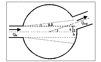
Figure: Manhole with one inlet, one outlet and a change in flow direction.

In the case of a change in flow direction, the effect of the jet at the outlet will gradually diminish with increasing angle. The effective flow area is therefore linearly interpolated between the full cross section area of the node, A, and the area of the jet, A_jet, as the angle increases.

The distance, a, from the point where the jet intercepts the node to the centreline of the inlet, see the manhole with one inlet, one outlet and a change in flow direction, is conservatively calculated as half the diameter of the inlet, D_in, thus neglecting the entrainment angle of 6.8°.

\[ a=\frac{D_{i n}}{2} \]

Equation: Distance from jet impingement to inlet centerline as half the inlet diameter.

The distance, b, from the point where the side of the outlet enters the node to the centreline of the inlet, is approximated with:

\[ b~=~\mathrm{max}\Bigl(0.0,\frac{D}{2}\cdot\tan\Bigl(\frac{\theta}{360}\cdot2\pi\Bigr)-\frac{D_{o u t}}{2}\Bigr) \]

Equation: Distance from outlet entry point to inlet centreline accounting for deflection angle.

where q is the angle between the centrelines of the inlet/outlet and D_out is the diameter of the outlet reach.

In the case of a change in elevation the effective flow area is diminished with a factor, drop_factor, which is equal to 1 when the inlet flows directly into the outlet and 0 when there is no interception between the incoming jet (calculated conservatively without the entrainment angle) and the outlet. In between these two conditions the drop factor is interpolated linearly.

The effective flow area is then interpolated as:

\[ A_{fl} = A_{jet} \cdot \left(1-\frac{b}{a}\right) \cdot \text{drop\_factor} + \left(1-\left(1-\frac{b}{a}\right) \cdot \text{drop\_factor}\right) \cdot A_{fl} \]

Equation: Effective flow area interpolated between jet area and full cross-section based on jet interception.

For a straight inlet/outlet with no change in elevation the formula gives that the effective flow area equals the jet area.

Headloss calculation for outflowing water

Headloss as water flows out of a node is calculated separately for each outlet link. The outlet loss for the link j is assumed to be proportional to the velocity head in the outlet link j:

\[ \Delta E_{j}~=~{\sum_{k}}\zeta_{j k}~{\cdot}~{\frac{v_{j}^{2}}{2g}} \]

Equation: Outlet headloss as sum of individual link headlosses proportional to outlet velocity head.

where x_jk are individual headloss coefficients for link j, calculated on the basis of the geometry of the node and flow distribution among the links attached to the node.

Loss due to change in flow direction

This loss is a function of the angles between the inlet and outlet links and distribution of the discharge in the inlet and outlet links, as shown in the example of manhole with two inlets and one outlet and the example of manhole with one inlet and two outlets.

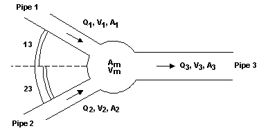
Figure: Example of manhole with two inlets and one outlet.

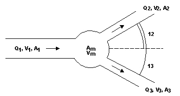
Figure: Example of manhole with one inlet and two outlets.

Based on the generalised notation, the calculation of the headloss coefficient is performed individually for each outlet link as follows:

\[ \zeta_{dir(j)} = \sum_{i=1}^{n} \frac{Q_i}{Q_{totalOut}} \cdot \frac{\theta_{ij}^2}{90^{\circ 2}} \]

Equation: Direction-based headloss coefficient accounting for flow angle distribution and momentum splitting.

where i stands for inlet links, and j stands for outlet links.

Loss Due to Change in Elevation

Vertical changes in flow direction occur and cause energy losses if there is a difference in elevation between the inlet and outlet links. These losses are described considering the magnitude of the difference in elevation, see the manhole with a difference in elevation between inlet and outlet pipe.

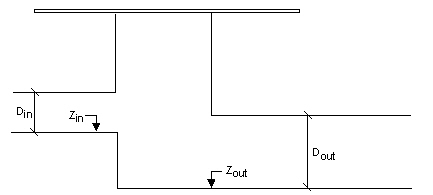
Figure: Manhole with a difference in elevation between inlet and outlet pipe.

The individual headloss coefficient is calculated according to the following expression, where the weighting relative to the flow rates in the inlet links relative to the outlet link is also included:

\[ \zeta_{level(j)} = \sum_{i=1}^{n} \frac{Q_i}{Q_{totalOut}} \cdot \frac{(Z_i - Z_j) \cdot (Z_j + D_j - Z_i - D_i)}{D_i \cdot D_j} \]

Equation: Headloss coefficient at a node weighted by inlet flow rates and elevation differences.

If the calculated headloss coefficient is smaller than 0, a zero value is assumed.

Loss Due to Contraction

The flow leaving the manhole and entering the outlet conduit is more or less contracted and due to subsequent expansion there occurs an energy loss. The outlet headloss coefficient depends on the shape of the manhole outlet, manhole and the link cross sections and distribution of flow among multiple inlet and outlet links.

The outlet headloss coefficient are calculated as:

\[ \zeta_{c o n t(j)}=~\operatorname*{min}\left[1,k_{m}\left[1-\frac{A_{j}}{A_{m}\cdot\frac{Q_{j}}{n}}{\sum_{i-1}}Q_{i}\right]\right] \]

Equation: Outlet contraction headloss coefficient depending on area ratios and flow distribution.

where:

K_m         =   specified outlet 'shape' coefficient for the node. For relatively large basins, K_m approaches z_contr. A_m=   flow cross sectional area in the node.

Limiting the contraction headloss to 1 helps to ensure numerical stability.

Limiting the total headloss for outflowing water

Theoretically, the total energy loss at the outlet from the node, expressed as a function of the velocity head in the outlet pipe can be as high as the available energy level in the node. The limiting case occurs e.g. with a completely clogged outlet (K_m -> ¥), with no flow in the outlet pipe.

To ensure numerical stability of the computation, the maximum headloss is limited to the depth in the outlet pipe:

\[ \Delta E_{j} = \text{min}\left(h_{j}, \left(\left(1 + \zeta_{out}\right) \cdot \frac{v_{j}^{2}}{2g} -\frac{v_{m}^{2}}{2g}\right)\right) \]

Equation: Maximum allowable headloss at outlet limited by available energy or outlet depth.

Selecting an appropriate local headloss computation

Urban (MIKE+)

This entire section applies to MIKE+ type setups only.

In some cases, results from using different approaches for headloss calculation can differ considerably, and due attention must be paid to the selection of the most appropriate approach.

The headloss calculation for individual nodes can be controlled by selecting one of five available options.

Each option is characterised by the fundamental computational principle and by a number of parameters which control the behaviour of the algorithm or the size of loss coefficient. In MIKE+, the existing options can be modified and new options created in “Outlet Headloss” dialog. Furthermore, the actual headloss calculation for individual nodes can be controlled by a local specification of various relevant parameters.

Constitutive Parameters of Headloss Computation Options

The following parameters constitute a definition of headloss calculation option:

Computation Method

Three different methods are available:

• MOUSE Classic (Engelund)
• Weighted Inlet Energy Method
• No Headloss Calculation

The first two are described in detail above in Section 4.6.2.

The third option ignores all local losses. Regardless of the shape of the outlets, the geometry of the junction or the distribution of flows among inlet and outlet conduits, water levels at the junction and the outlet conduit are set to the same value, as if there is no change in geometry and no change in the flow conditions between the junction and outlet conduit. This literary means that this option should be applied only where there is no change in cross section. If applied inappropriately, inconsistent results may be generated. This option can be recommended for use if an artificial node is introduced somewhere on a straight section of a reach, where no actual losses occur.

Maximum Loss Limit

This parameter is of relevance for both MOUSE Classic and Weighted Inlet Energy computation methods. It limits the maximum computed headloss to the water depth or the velocity head in the outlet pipe, according to Section 4.6.4.

Loss Coefficient

The available loss coefficient types distinguish three different interpretations of the specified headloss coefficient.

Selection of “K_m”(Type (a)) interprets the specified value as the outlet 'shape' coefficient Km (see Equation the outlet contraction headloss coefficient depending on area ratios and flow).

Selection of “Contraction HLC” (Type (b)) interprets the specified value as the outlet 'contraction' coefficient zcontr(j) (see Equation the outlet contraction headloss coefficient depending on area ratios and flow). This means that the model ignores the geometrical relations between the node and the outlet links (outlet shape), and applies the specified value directly as the zcontr. The contraction losses in the outlet links are then computed by multiplying the velocity head in the respective link by the zcontr. The total headloss for an outlet link is computed as a sum of the contraction, direction and elevation loss.

Selection of “Total HLC” (Type c)) interprets the specified value as the total outlet headloss coefficient (z_out). This means that the model completely ignores the geometry of the node/links, and applies the specified value (Total HLC) directly as the z_out, the same for all outlet links at the node. The total headlosses in the outlet links are then computed by multiplying the velocity head in the respective link by the specified z_out.

Effective Node Area

This parameter is only relevant for the MOUSE Classic computational method and for flow-through manholes in circular pipes. In all other cases, the default total wetted node area is applied. The following choices are available:

• Total wetted node area: calculated as product of the diameter and water depth for manholes and read from the basin geometry table (A_c) for basins. Typically results in overestimation of local headloss in a node
• Calculated Effective Area: the effective area in a manhole is calculated on the basis of empirical formula (see Section 4.6.2 Headloss calculation for inflowing water (p. 58)). This results in a significantly smaller area than the full wetted area and, consequently, in a more realistic flow calculation
• Reduced Calculated Effective Area: the effective area in a manhole is further reduced to 50% of the calculated effective area

Default Computational Options

The following tables provide an overview of available headloss calculation options in MOUSE and MIKE+. By comparing the two tables, it is possible to identify the equivalent options. During the import of a MOUSE project into MIKE+, the nine options are imported under their original names with the prefix “MOUSE_”.

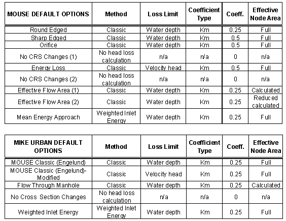
Figure: Headloss options in MOUSE and MIKE+.

Example: Variation in Node Outlet Headlosses as a Function of the Headloss Coefficient Mode

In this example a simple sewer system consisting of two pipes, two manholes and one outlet is constructed. Tests for different types of headloss (a), (b) and (c) have been performed with various modifications in flow direction or drop height, or both. the test matrix for implementation of Headloss Type shows a complete test matrix.

Four variants of the model setup have been constructed:

I)         Straight sewer pipelines with no drops and no changes in directions.

II)      A change in direction is introduced in variant I).

III)   A drop is introduced in variant I).

IV)   A drop and a change of direction are introduced in variant I).

A definition sketch of the setups I)-IV) is shown in the sketch to define the various terms of the example. The manual calculation example corresponds to test No. 4 in the test matrix.

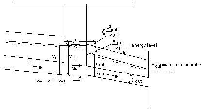
Figure: Sketch to define the various terms of the example.

In the performed tests, the value of the HEADLOSS COEFFICIENT has been set to 0.5 for all three types (a), (b) and (c). The headloss coefficients for a drop in the setup III) and IV) is 0.4 (inlet pipe is 0.6 m above the bottom in manhole B). The headloss for the direction in the setup II) and IV) is 0.25 (angle between pipes are 45°).

The example also includes the calculation of the friction loss in the downstream pipe.

Manual Headloss Calculation

Assumptions:. The water level in the inlet pipe is assumed to be equal to the water level in the manhole. This implies that the expansion loss at the inlet is automatically assumed. All calculated energy losses are assumed to occur at the outlet pipe, i.e.:

\[ E_{manhole} = E_{pipe} + \Delta H \]

Equation: Energy balance relating manhole energy level to outlet pipe energy and headloss.

or expressed by using the notation in the sketch to define the various terms of the example:

\[ \frac{v_{m}^{2}}{2g}\!+\!y_{m}\!+\!Z_{m}\!=\frac{v_{o u t}^{2}}{2g}\!+\!y_{o u t}\!+\!Z_{o u t}\!+\!\zeta\frac{v_{o u t}^{2}}{2g} \]

Equation: Energy balance equation for headloss calculation in a manhole with velocity and elevation terms.

z   =   a coefficient expressing the total outlet energy loss (see Section 4.6.3 Headloss calculation for outflowing water (p. 60)).

Data:

Discharge                     Q   =   2.0   m³s^-1 Diameter in outlet pipe                     D_out   =   1.0   m Diameter in manhole                     D_m   =   1.5   m Velocity in outlet pipe (Q is capacity assumed)                     V_out   ~   2.55   ms^-1 Length of outlet pipe                     L   =   50.0   m Manning number                     M   =   70   m^1/3s^-1 Water level in outlet                     H_out   =   15.0   m Bottom level in manhole                     Z_m   =   14.0   m Head “shape” loss coefficient                     K_m   =   0.5

Friction loss in outlet pipe from manhole to outlet:

\[ h_{f} = \frac{Q^{2}L}{M^{2}A^{2}R^{\frac{4}{3}}} = \frac{2.0^{2} \cdot 50.0}{70^{2} \cdot 0.7854^{2} \cdot 0.25^{\frac{4}{3}}} \]

Equation: Friction head loss in an outlet pipe from manhole using Manning equation with discharge, length, and geometry.

The water level in the manhole (H) can be found from:

\[ H + \frac{v_m^2}{2g} = H_{out} + h_f + \frac{v_{out}^2}{2g} + \zeta \frac{v_{out}^2}{2g} \]

Equation: Energy balance in a manhole node with velocity and friction head terms.

v_m is approximated by assuming that y_m = y_out:

\[ v_{m} = \frac{Q}{A_{m}} = \frac{Q}{D_{m}y_{m}} = \frac{2.0}{1.5 \cdot \left(15.0 + 0.42 -14.0\right)} = 0.94ms^{-1} \]

Equation: Example calculation of flow velocity in a manhole chamber.

\[ v_{out} = \frac{Q}{A_{out}} = \frac{2.0}{0.78} = 2.55 ms^{-1}, \quad \frac{v_{out}^2}{2g} = 0.33 m \]

Equation: Outlet velocity and velocity head computed from discharge and outlet area.

\[ \frac{v_{m}^{2}}{2g}~=~0.045~\mathrm{m} \]

Equation: Velocity head calculation at manhole node from discharge and cross-sectional area.

\[ \zeta = \zeta_{contr} + \zeta_{dir} = K_m \cdot \left(1 - \frac{A_{out}Q_{in}}{Q_{out}A_m}\right) + \frac{Q_{in}}{Q_{out}} \cdot \frac{\theta^2}{90^2} = 0.5 \cdot \left(1 - \frac{0.78}{1.5 \cdot 1.42}\right) + \frac{45^2}{90^2} = 0.567 \]

Equation: Combined contraction and directional loss coefficient from geometric and discharge properties.

Substituting values to the Equation the example calculation of flow velocity in a manhole chamber and calculating H yields:

\[ H~=~15.89~\mathrm{m} \]

Equation: Calculated water level in manhole from energy balance and headloss terms.

The deviation between the MOUSE simulation and manual calculation result is due to the fact that MOUSE calculates v_out by using the following area in the pipe:

\(A_{out} = \frac{D_{out}^2 \pi}{4} + \text{Preismann slot area}\) 

The table shows which setups have been used for the calculation, and also which types of headloss are included. z_c0, z_c1, z_c2 are all headloss coefficients due to contraction and correspond to the types (a), (b) and (c).

Table: Test matrix for implementation of Headloss Type.

Test	Setup	Direction zd	Drop zl	Contraction zc (a) zc0	Contraction zc (b) zc1	Contraction zc (c) zc0	Hcalc	HM
1	I)			X			15.81	15.82
2	I)				X		15.87	15.87
3	I)					X	15.87	15.87
4	II)	X		X			15.89	15.90
5	II)	X			X		15.95	15.94
6	II)	X				X	15.87	15.87
7	III)		X	X			15.94	15.94
8	III)		X		X		16.00	15.99
9	IV)	X	X	X			16.02	16.02
10	IV)	X	X		X		16.03	16.02