Adaptive Time Step Size
The computational efficiency of any discrete-time numerical simulation algorithm is highly dependent on the time step size applied in the simulations.
In turn, the feasible time step in a concrete situation depends on the inherent performance properties of the computational scheme and the dynamics of the flows in the simulated network. It is therefore desirable to optimise the algorithm so that in conditions of variable flow dynamics, the total computational effort is minimised, while preserving stable and accurate computations.
The 1D engine includes three modes of time step size control: Fixed, tabulated and adaptive.
Fixed time stepping is the traditionally used time stepping where a time step is specified as input and used throughout the simulation period.
In the tabulated time step mode, time step sizes are given as a time series. Tabulated time stepping is especially useful when studying events that occur at a certain time that is known in advance of the simulation. For instance a dambreak known to occur at a certain date and time or a massive inflow occurring in a certain month every year due to a rainy season, etc.
The adaptive time stepping is used for modelling scenarios where the preferred time step is not known in advance. The adaptive time step may be used for obtaining a more detailed modelling of certain critical parts of a simulation, typically parts where large changes appear or it may be used for preventing calculations to blow up due to numerical instabilities.
Adaptive time stepping adjusts the time step size to be between a minimum and maximum time step size, both user specified. A number of checks on the boundary values and the solution are used during the simulation to adjust the time step size. All checks are optional.
Adaptive time stepping can be applied to Dynamic and Diffusive flow descriptions, but it cannot be used with the Kinematic flow description.
The remainder of this section presents details of how adaptive time stepping determines the time step size.
Adaptive step size methodology
In the 1D engine adapts the time step size in a two step process:
First, before every time step, the preferred time step is calculated based on boundary checks and the solution from the last time step. For every solution check, a factor is calculated that defines how much the time step can be increased in order for the check still to be valid. If the solution evaluates to only half of the check limits, the time step size can be doubled (the factor will be 2).
The smallest of the factors from all solution checks is used to calculate the preferred time step. The new time step size is the factor times the time step size of the last time step times a buffer factor. The buffer factor is between 0.95 and 0.99.
Second, the time step is performed. If one or more of the solution checks are not fulfilled, then the time step is rejected and the time step decreased (at least by a constant factor), and the time step is performed again with the new time step.
This methodology is different from the one employed in MIKE+. Chiefly, in MIKE+, if a check fails, then the actual solution is a linear interpolation of the prior solution and the new solution for which the check failed. The methodology in the 1D engine is superior to the MIKE+ methodology since the calculated solution is not based on linearly interpolating a result which failed the checks, and therefore the net accuracy is higher. The result is that the 1D engine performs fewer time steps than MIKE+ while retaining the same or higher accuracy.
This methodology is different from the one employed in MIKE 11. Chiefly, in MIKE 11, the time step size is increased by a constant factor before each time step. If a check fails, then the solution is discarded and the time step is re-calculated. The methodology in the 1D engine is superior to the MIKE 11 methodology since substantially fewer time steps are re-calculated.
Boundary value check
The check on the boundaries helps avoiding input details to be neglected due to application of too large a time step. The boundary check limits the acceptable relative difference between the boundary value obtained by linear interpolation between two solution times, t and t+Dt, and the actual boundary value given in the boundary time series. The difference is calculated at three points in the t to t+Dt interval. If the maximum of these three values divided by the interpolated value is larger than acceptable relative difference, then the time step is too large. the black line is the actual boundary values and the dashed line is the linearly illustrates this principle.
Since this is a check on the relative value of the boundary, it is only active if the boundary value at t+Dt is larger than a specified minimum value.
This sampling criteria used when checking boundaries is very general and is applied to all types of boundaries.
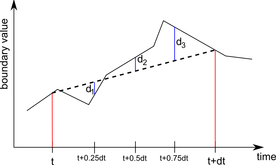
Figure: The black line is the actual boundary values and the dashed line is the linearly interpolated boundary used in the simulation.The maximum of the differences d1, d2, and d3 relative to the boundary value is limited by the boundary value check.
In MIKE+, the maximum allowed relative variation is QacceptLimitRel, and the specified minimum value for the check to be active is QlowLimitM3s, both from the dhiapp.ini file.
The default value of QacceptLimitRel is 0.1 and QlowLimitM3s 0.01.
In MIKE 11, the maximum allowed relative variation is resid(BC)/BC, and the specified minimum value for the check to be active is BC, both from the Time Step Settings dialog window.
Solution check: Discharge variation in grid points
Two check are performed on the discharge in q-grid points. First, the variation in discharge must be below a specified value:
Equation: Discharge variation solution check criterion for adaptive time stepping.
Secondly, the relative variation in discharge must be below a specified value:
\(\left|\frac{\Delta Q}{Q}\right| < val_{qRel} \quad \text{for} \quad |Q| < limit\)
This check is not available in MIKE+
In MIKE 11, valq is delQ, valqRel is delQ/Q, and limit is Q, all from the Time Step Settings dialog window.
Solution check: Water level variation in grid points
Two checks are performed on the water level in h-grid points. First, the variation in water level must be below a specified value:
Equation: Stability criterion limiting absolute water level variation within a time step.
Secondly, the relative variation in water level must be below a specified value:
\(\left|\frac{\Delta h}{d}\right| < val_{hRel} \quad \text{for} \quad |d| > limit\)
where d is the water depth.
In MIKE+, the variation in water level check is not performed. The relative water level check is performed, but d is the height of the cross section at that h-grid point, and the limit is applied to the relative depth. In addition, if the relative change in water level is below limit, then valhRel and limit are adjusted down as a function of relative depth, with a minimum value of 0.02.
Both valhRel and limit are WaterLevDiffMaxRel from the dhiapp.ini file
The default value of WaterLevDiffMaxRel is 0.3.
In MIKE 11, valh is delh, valhRel is delh/h, and limit is h, all from the Time Step Settings dialog window.
Solution check: Water level variation in nodes
The check on water levels in nodes is actually a check on all connections into the nodes. The check is active only if water flows from the connecting reach into the node. In addition, the following two conditions must be true. First, the water level in the grid point closest to the node at time n+1 plus 0.05 must ne smaller than the water level in the node at time n+1 (time n+1 refers to the most recent values, while time n are the values of the previous time step). In an equation it can be written as:
\(h_{n p~1,~g p}+0.05<h_{n p1}\)
Second, the water level in the grid point at time n must be larger than the water level in the node:
\(h_{np1} -h_{n}\),
where h is water level, n and n+1 refer to the time step, and gp is for grid point.
If these three conditions are all true, and
\(h_{n p~1,~g p}-h_{n,~g p}+0.05<h_{n p~1}-h_{n}\)
then the time step is adjusted with a factor of
\(\frac{h_{n p1,g p}-h_{n,g p}+0.05}{h_{n p1}-h_{n}}\)
This check is not available in MIKE 11.
Solution check: Courant value
There are two types of checks on the Courant number. An “HD” Courant check:
Equation: Courant number stability criterion for hydrodynamic flow conditions.
and an “AD” Courant check:
\(\left|Cr_{AD}\right| = \frac{|v|\Delta t}{\Delta x} < val_{AD}\)
where v is the flow velocity, Dx is the grid spacing, g is acceleration due to gravity, and D is flow area divided by flow width.
In MIKE+, only the “AD” Courant check is performed. valAD is MaxCourant from the dhiapp.ini file.
The default value of MaxCourant is 20.
In MIKE 11, valHD is Courant(HD), valAD is Courant(AD), both from the Time Step Settings dialog window.
Solution check: Pumps
Pumps can influence the time step size, but only of the flow calculation through the pump is explicit. Implicit pumps do not influence the time step size.
If the pump is either acceleration or decelerating, then the time step size is set to
\(\Delta t\!=\!\Delta t_{m i n}\!+\!f_{p u m p}(\Delta t_{m a x}\!-\!\Delta t_{m i n})\)
where \(\Delta t_{m i n}\) and \(\Delta t_{m a x}\) are the lower and upper limits on the time step
size, respectively, and \(f_{p u m p}\) is a user specified constant.
If the pump is not either acceleration or decelerating, then the time step is adjust if
\(\left|q_{n p1}-q_{n}\right|>\frac{0.05q_{n p1}\Delta t_{m i n}}{\Delta t_{n}-\Delta t_{m i n}}\)
where \(\Delta t_{n}\) is the previous time step. If this condition is true, then the time
step is set to
\(\Delta t~=~\Delta t_{m i n}\!\left(1.0+\frac{0.05q_{n p1}}{\left|q_{n p1}\!-\!q_{n}\right|}\right)\).
In MIKE+, \(f_{p u m p}\) is PumpAccDecVarDtRel from the dhiapp.ini file.
The default value of PumpAccDecVarDtRel is 0.
The check is not available in MIKE 11
Solution check: Cross section parameters
Variation in the cross section parameters A, R2/3 and B, where A is the cross section area, R is the hydraulic radius and B the width of water surface can influence the time step size. If the check is active then the cross sections is all h-grid points are checked.
These check are active only if the relative water depth in the cross section is larger than a user specified limit.
The variation in the three cross section parameters is limited by:
Equation: Permissible variation limit in cross-section parameters relative to maximum values.
where the variable X is one of the three cross section parameters and the meaning of Max(X) is either the maximum possible value of that parameter, or the actual value (user configurable). \(f_{XS}\) is a user specified constant.
If the check not true, then the time step size is adjusted by a factor of
\(\frac{\Delta X}{f_{XS} \cdot Max\left(X\right)}\).
In MIKE+, the limit value on the relative depth for whether the check is active is CrossLowDepthLimit from the dhiapp.ini file. The factor \(f_{XS}\) is MaxVarCrossConstant from the same file. Whether Max(X) refers to the maximum value or the actual value of the cross section parameter is controlled by Crosscheck from the dhiapp.ini file. If Crosscheck is 1, then the maximum value is used. If Crosscheck is 2, then the actual value is used. If Crosscheck is 0 then the checks are disabled.
The default value of MaxVarCrossConstant is 0.03, of Crosscheck it is 1 and of CrossLowDepthLimit it is 0.04.
The check is not available in MIKE 11