Linear Reservoir Surface Runoff Model
Concept
The Linear reservoir surface runoff computation of MIKE 1D is founded on the linear reservoir equations for routing the runoff through the catchment. This means that the surface runoff from a catchment is made proportional to the current water depth. In addition to the linear reservoir model, a French localised version has also been implemented.
The runoff amount is controlled by the initial losses, size of the actually contributing area and by infiltration losses. The shape of the runoff hydrograph (phase and amplitude) is controlled by the catchment time constant.
Input data
Model data are split into the global model and the French localised version.
Model-specific data
Global model
Effective area [-] represents the fraction of the catchment area considered to contribute effectively to the runoff.
French model (FR)
Impervious area [-] represents the fraction of the catchment area considered to contribute to the runoff. Calculations of the infiltration and the runoff will differ depending on value of the parameter:
Impervious area \(\geq\) 0.2: catchment is urban
Impervious area < 0.2: catchment is rural
Length [m] represents the estimation of the maximum runoff length from the periphery of the catchment to the point of connection used in the empirical calculation of the catchments lag time constant
Slope [-] represents the estimation of the average runoff slope used in the empirical calculation of the catchments lag time constant.
Hydrological parameters
Global model
Initial Loss [m] defines the precipitation depth required to start the surface runoff. This is a one-off loss, comprising the wetting and filling of catchment depressions.
The default value is 5.00 10-4 m.
Time constant [s-1] is the linear reservoir time constant controlling the shape of the runoff hydrograph (reaction time).
The default value is 3.00 10-3 s-1.
French model (FR)
The reduction factor [-] accounts for various hydrological losses not accounted explicitly in the computation.
The default value is 0.90.
The lag time [s] is the reciprocal equivalent of the linear reservoir time constant.
The default value is 300 s.
Infiltration
Start Infiltration rate [m/s] defines the maximum rate of infiltration (Horton) for the specific surface type.
The default value is 0.50 10-6 m/s.
End Infiltration rate [m/s] defines the minimum rate of infiltration (Horton) for the specific surface type.
The default value is 0.14 10-6 m/s.
Wet Horton exponent [s-1] is the time factor “characteristic soil parameter” used in the Horton’s equation. It determines the infiltration capacity rate reduction during rainfall.
The default value is 8.30 10-4 s-1.
Dry Horton exponent [s-1] is the time factor used in the “inverse Horton's equation”, defining the rate of the soil infiltration capacity recovery after a rainfall, i.e. in a drying period.
The default value is 0.28 10-4 s-1.
Recommended parameter values for various types of catchments are presented in the recommended values of parameters for Linear reservoir model for various types of catchment surfaces.
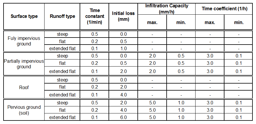
Figure: Recommended parameter values for the linear reservoir model for various types of catchment surfaces.
Runoff computation
The runoff computations are based on the volume continuity and the linear reservoir equations.
The first step is the calculation of the effective precipitation intensity. The effective precipitation intensity is the precipitation, which contributes to the surface runoff. Next, the hydraulic routing based on the linear reservoir principle and volume continuity is applied.
The localised version proposed a different calculation of the losses and the hydraulic routing. Three different types may be used:
-
Global model
-
French Urban model
-
French Rural model
The Impervious area input is the parameter used in the rule deciding whether a French catchment is Urban and Rural.
The hydrologic and hydraulic processes involved are shown in the diagram in the processes simulated in the Linear reservoir surface runoff model.
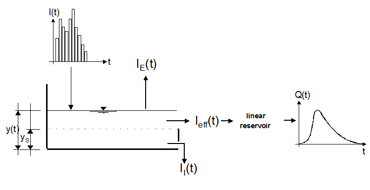
Figure: The processes simulated in the Linear reservoir surface runoff model.
Effective precipitation computation
The simulated hydrologic processes account for the losses - evaporation, infiltration and surface storage - calculated according to the conventions and equations in the order presented below. The remaining precipitation is called effective precipitation, defined generally as:
Equation: Effective precipitation after accounting for evaporation, infiltration, and surface storage losses.
Where:
Table: Variables in the effective precipitation equation.
| \(I(t)\) | Actual precipitation intensity at time t |
| \(I_{E}(t)\) | Evaporation loss at time t. It should be noted that the evaporation loss for the catchment is accounted only if the evaporation explicitly is activated. Otherwise, it is replaced by a constant decay rate |
| \(I_{s}(t)\) | Initial loss (wetting and surface storage) at time t |
| \(I_I(t)\) | Accumulated depth at time t |
The individual terms in the loss equation are fundamentally different, as some terms are continuous where others are discontinuous. If the calculated loss is negative, it is set to zero. The losses have a dimension of velocity [LT-1].
The actual precipitation, I(t), is assumed to be uniformly distributed over the individual catchments. Otherwise, it may vary as a random time function.
The surface storage, IS(t), is the loss due to wetting and filling the depressions and holes in the terrain. The model begins with the surface storage calculation after the wetting process is completed. The surface storage is filled only if the current infiltration rate is smaller than the actual precipitation intensity reduced by evaporation. The actual surface storage loss is calculated according to the following:
Equation: Surface storage loss as the difference between precipitation and infiltration when storage is unsaturated.
Where:
Table: Variables in the surface storage loss equation.
| \(I(t)\) | Precipitation intensity at time t |
| \(I_{s}(t)\) | Surface storage loss at time t |
| \(I_I(t)\) | Infiltration loss at time t |
| \(I_{E}(t)\) | Evaporation loss at time t |
| ys | Surface storage depth |
| \(y(t)\) | Accumulated depth at time t |
The infiltration, II(t), is the water loss to the lower storage caused by the porosity of the catchment surface. It is assumed that the infiltration starts when the wetting of the surface has been completed. The infiltration loss is calculated according to the following relations:
Equation: Infiltration loss to lower storage zone bounded by maximum infiltration rate.
Where:
Table: Variables in the infiltration loss equation.
| \(I_I(t)\) | Infiltration loss at time t |
| \(I_H(t)\) | Horton’s infiltration at time t (see below)* * |
By default the infiltration is taken into account in the calculation if the option is activated. However, the French Urban catchment will disregard any infiltration, even if it has been activated.
Valid for Global and French Rural models, only: The infiltration is a complex phenomenon, dependent on the soil porosity, moisture content, groundwater level, surface conditions, storage capacity, etc. The model calculates the infiltration loss capacity using the well-known Horton’s equation, per default in its original form:
Equation: Horton infiltration capacity decay with exponential time dependence.
Where:
Table: Variables in Horton's infiltration capacity equation.
| \(I_H(t)\) | Infiltration loss calculated according to Horton |
| \(I_{Imax}\) | Maximum infiltration capacity (at start) |
| \(I_{I m i n}\) | Minimum infiltration capacity (at full saturation) |
| t | Time since the start of the storm |
| ka | Time factor (characteristic soil parameter) for wetting conditions |
By default the model is able to calculate the infiltration following the standard and the integrated form of Horton’s equation. However the French rural model only offers the possibility to calculate the infiltration only according to the standard form.
Valid for Global model, only (not valid for the French model): The Horton's equation in its original form, Equation the horton infiltration capacity decay with exponential time dependence, yields in realistic results only if applied to events for which the rainfall intensity always exceeds the infiltration capacity. However, typical values for infiltration capacity parameters IImax and IImin are often greater than typical rainfall intensities. Thus, when Equation the horton infiltration capacity decay with exponential time dependence is used, with infiltration capacity IH being the function of time only, IH will decrease even if rainfall intensities are very small. In other words, this results in a reduction in infiltration capacity regardless of the actual amount of water entering the soil. This problem is solved by implementing the integrated form of the Equation the horton infiltration capacity decay with exponential time dependence:
Equation: Cumulative infiltration over time combining minimum rate and exponential decay component.
Where:
Table: Variable in the cumulative infiltration equation.
| ICUM(tp) | A cumulative infiltration (m) at time tp, i.e. the area under the Horton's curve |
This assumes that the actual infiltration has been equal to the infiltration capacity at any time within the period 0->t. Since this is only the case for rainfall intensities higher than the infiltration capacity, this needs to be corrected as:
Equation: Cumulative infiltration computed by integrating infiltration rate over time.
i.e. the cumulative infiltration at the elapsed time t is calculated using the actually occurred infiltration.
At any elapsed time t, the two equations the cumulative infiltration over time combining minimum rate and exponential decay and the cumulative infiltration computed by integrating infiltration rate over time can be used to determine the “equivalent” time tp. This is done iteratively, since equation the cumulative infiltration over time combining minimum rate and exponential decay cannot be solved explicitly for tp.
The time tp on cumulative Horton's curve will always be less or equal than the actually elapsed time, implying that the available infiltration capacity at time tp will be greater than or equal to that given by the equation the horton infiltration capacity decay with exponential time dependence. By these means, the infiltration capacity has been made a function of actual water infiltrated and not just a function of time.
Application of a “standard” Horton's equation the horton infiltration capacity decay with exponential time dependence or its integrated form (equations the cumulative infiltration over time combining minimum rate and exponential decay and the cumulative infiltration computed by integrating infiltration rate over time) is controlled by the switch IntegratedHorton, found in INI file (see relevant documentation for reference). Per default, the program is set to “standard” Horton's equation.
In the dry period following the rainfall, the infiltration capacity is gradually recovered to the initial value, using an inverse form of the Horton's equation:
Equation: Infiltration capacity recovery in dry period following rainfall using inverse Horton equation.
Where:
Table: Variable in the cumulative infiltration equation.
| \(I_H(t)\) | Infiltration loss capacity calculated according to Horton |
| \(I_{Imax}\) | Maximum infiltration capacity (after a long dry period) |
| \(I_{IT}\) | Infiltration capacity at the threshold between the wetting and drying period |
| t | Time since the start of the recovery process |
| kh | Time factor (characteristic soil parameter) for drying conditions |
The evaporation, IE(t), is a continuous loss that is normally of less significance for single event simulations. However, on a long-term basis, evaporation accounts for a significant part of hydrological losses. If included in the computation, the evaporation is the first part subtracted from the actual precipitation, according to the following:
Equation: Evaporation as either actual evaporation demand or actual precipitation depending on rainfall and water availability.
Where:
Table: Variables in the evaporation loss equation.
| \(I_a(t)\) | Actual precipitation at time t |
| \(I_{E}(t)\) | Evaporation loss at time t |
| \(I_{PE}(t)\) | Potential evaporation at time t |
| \(y(t)\) | Accumulated depth at time t |
If the evaporation has not been explicitly included in the simulation (i.e. evaporation process is activated and a time series is included), a constant decay rate is applied instead (see Section 7.5.4).
Surface Runoff routing computation
The runoff starts when the effective precipitation intensity is larger than zero. The hydraulic process is described with the linear reservoir equation.
Linear reservoir equation
The surface runoff at time t is calculated as:
Equation: Surface runoff discharge from linear reservoir proportional to storage raised to the 5/3 power.
Where:
Table: Variables in the linear reservoir discharge equation.
| C | Linear reservoir constant |
| \(y_{R}(t)\) | Runoff depth at time t |
The depth yR(t) is determined from the continuity equation:
Equation: Continuity equation for runoff depth relating effective precipitation to discharge.
Where:
Table: Variables in the runoff depth continuity equation.
| Ieff | Effective precipitation |
| A | Contributing catchment surface area |
| dt | Time step |
| \(d y_{R}\) | Change in runoff depth |
Linear reservoir constant By default, the linear reservoir constant C is equal to the catchment time constant.
The French model calculates the constant is in different ways. The reservoir constant is calculated as follow:
If the lag time is greater than 10-5 s:
Equation: Reservoir routing constant computed from basin lag time.
Where:
Table: Variable for catchment lag time constant.
| TL | Catchment lag time |
Otherwise, the model provides an empirical formula for the calculation of the reciprocal value K (= 1 / C) of the reservoir constant C as:
Equation: Empirical formula for catchment lag time constant based on area, rainfall, slope, and length.
The lag time is corrected depending on imperviousness and size:
- for Urban catchment: \(K_{C}=~0.5\cdot K\)
- for Rural catchment:
- \(\mathrm{A}<6~\mathrm{ha}:K_{C}~=~0.8\cdot K\)
- \(6\leq A<250~\mathrm{ha}:K_{C}~=~0.7\cdot A^{-0.009}\cdot K\)
- \(\mathbf{A}\geq250~\mathrm{ha}:K_{C}=K\)
Where:
Table: Equation parameters and variables.
| A | Total catchment surface area (ha) |
| I | Impervious part of the catchment (0…..1.0) |
| S | Catchment slope (%) |
| L | Catchment length (m) |
Surface runoff computation
A single linear reservoir equation is applied by default.
\(Q(t_i) = Q(t_{i-1})e^{-C \cdot dt} + Q_i(t_i) \cdot (1 - e^{-C \cdot dt})\)
For the French Rural catchment the double linear equation is applied.
\(\begin{array}{l} Q_1(t_i) = Q_1(t_{i-1})e^{-C \cdot dt} + Q_i(t_i) \cdot (1 - e^{-C \cdot dt}) \\ Q(t_i) = Q(t_{i-1})e^{-C \cdot dt} + Q_1(t_i) \cdot (1 - e^{-C \cdot dt}) \end{array}\)
Where:
Table: Variables for catchment lag time corrections based on size and impervious area.
| \(Q(t_i)\) | Total runoff at time step ti |
| \(Q(t_{i-1})\) | Total runoff at previous time step ti-1 |
| \(Q_1(t_i)\) | Outflow of the intermediate reservoir at time step ti |
| \(Q\left(t_{i -1}\right)\) | Outflow of the intermediate reservoir at previous time step ti-1 |
| C | Linear reservoir constant |
| dt | Time step length |
Multiple-event simulations
In order to speed up the calculations, a different time step is applied during dry periods and a special solution has been applied for the simulation of dry periods between the consecutive events. The solution accounts for the following phenomena:
In this context, start of a dry period is defined if three conditions are fulfilled simultaneously:
- No rainfall: all connected rain gauges show no rain, i.e. the rainfall intensity is null
- No infiltration: the infiltration has stopped in the catchment (and not necessary in all catchment like it is done in MOUSE)
- No runoff: the runoff from the catchment included in the simulation has fallen below the “low flow” limit. The threshold can be controlled through the parameter NL_CONCEPT_DRYDEPTH in the INI file (see relevant documentation for reference)
At the start of a dry period, the initial loss storage would appear fully or partially filled up. For flat impervious surfaces, the full initial loss storage would contain the water used for wetting and filling of the surface storage, while for all other surface types only wetting loss will apply. The latter case, i.e. partially filled storage would apply for small events with the total depth smaller than the corresponding initial loss storage capacity.
If evaporation is not specified, recovery of the initial loss capacity, i.e. the process of surface drying is simulated as a constant “decay” rate, which replaces the actual evaporation. As a consequence of the recovery process, the initial loss storage would be fully or partially emptied, which depends on the actually applied loss recovery rate and the duration of the dry period.
The initial loss recovery rate can be controlled through RUNOFF_C_INITLOSS_RECOVER found in the INI files (see relevant documentation for reference).
The recovery process is only activated during dry periods, i.e. the action during rain events is neglected. Note that if actual evaporation process is activated, the recovery process is suppressed and evaporative action is activated throughout the simulation period.