Unit Hydrograph Surface Runoff Model UHM

Concept

The UHM module simulates the runoff from single storm events for any number of catchments defined in the MIKE 1D model setup, by the use of the well-known unit hydrograph technique. As such, UHM constitutes an alternative to the other runoff models available in MIKE 1D, for the runoff simulation in the areas where no flow records are available or where unit hydrograph technique has already been well established.

The unit hydrograph model calculates the excess rainfall (precipitation) assuming that the losses to infiltration can be described as a fixed initial and constant loss, a proportional loss (the rational method) or by the U.S. Soil Conservation Service (SCS) curve number method or finally by the generalises SCS method.

The excess rainfall is routed by the unit hydrograph method. The module applies the SCS-dimensionless hydrographs or the Snyder Unit Hydrograph.

In order to setup a UHM model three sub models are to be defined:

• The loss model
• The hydrograph type
• The lag time model

The loss model

During a rainstorm, a part of the rainfall infiltrates to the soil. Subsequently, a large part of the infiltrated water evaporates, while only a relatively small fraction reaches the drainage network. Hence, in single-event models such as UHM, it is reasonable to describe the major part of the infiltration as a loss. The amount of precipitation actually reaching the sewer system, i.e. the total amount of rainfall reduced by the loss, is termed the excess precipitation.

The unit hydrograph model includes four optional methods for calculation of excess precipitation. They are all lumped models, considering each catchment as one unit and hence the parameters represent average values for the catchment.

All the methods include an area adjustment factor [-], accounting to some extent for a non-uniform distribution of precipitation over the catchment.

Proportional loss model (the rational method)

Input data

Input that must be set for this loss model: Runoff coefficient [-]

Loss computation

In this method the losses are assumed to be proportional to the precipitation rate and thus the excess precipitation is given by:

\[ P_{excess} = a \cdot A_{f} \cdot P \]

Equation: Excess precipitation from proportional loss model related to area factor and rainfall.

Where:

Table: Variables in the proportional loss model equation.

Pexcess	Excess precipitation (m/s)
a	User-defined runoff coefficient between 0 and 1
Af	Area adjustment factor
P	Precipitation rate (m/s)

SCS Loss Model

The U.S. Soil Conservation Service (SCS), /1/, developed this method for computing losses from storm rainfall in 1972.

Input data

Inputs that must be set for this loss model:

Initial antecedent moisture conditions (AMC) [-] Curve number [-]

Loss computation

For the storm as a whole, the depth of excess precipitation or direct runoff P_e is always less than or equal to the depth of precipitation P. Likewise, after the runoff begins, the additional depth of water retained in the catchment, F_a, is smaller than or equal to some potential maximum retention S (see the variables in the SCS method of rainfall abstractions: I_a = initial abstraction). There is a certain amount of rainfall I_a, (initial loss before ponding) for which no runoff occurs. Consequently, the potential runoff amounts to P - I_a.

The hypothesis of the SCS method is that the ratios of the two actual to the two potential quantities are equal, i.e.:

\[ \frac{F_{a}}{s} = \frac{P_{e}}{P -I_{a}} \]

Equation: SCS method hypothesis equating ratios of actual to potential runoff and infiltration.

The continuity principle results in:

\[ P~=~P_{e}+I_{a}+F_{a} \]

Equation: Continuity equation for SCS method partitioning rainfall into runoff, initial loss, and infiltration.

Combining Equations the SCS method hypothesis equating ratios of actual to potential runoff and and the continuity equation for SCS method partitioning rainfall into runoff, initial gives:

\[ P_{e}~=~\frac{\left(P-I_{a}\right)^{2}}{P-I_{a}+S} \]

Equation: Excess precipitation computed by the SCS Curve Number method.

which is the basic equation for computing the depth of excess precipitation or direct runoff from a storm by the SCS method.

The results from many small experimental watersheds were used to obtain an empirical relationship:

\[ I_a = 0.2S \]

Equation: Soil Conservation Service initial abstraction empirical relationship.

The basic equation used in this model is derived by combining Equations the excess precipitation computed by the SCS Curve Number method and the soil Conservation Service initial abstraction empirical relationship:

\[ P_{e}~=~\frac{\left(P-0.2S\right)^{2}}{P+0.8S} \]

Equation: Excess precipitation using SCS method from total rainfall and maximum retention parameter.

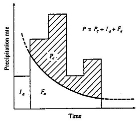
Figure: Variables in the SCS method of rainfall abstractions: I_a = initial abstraction, P_e = accumulated excess rain, F_a =  continuing abstraction, P = total rainfall.

The potential maximum retention S is calculated from a dimensionless curve number (CN) using the empirical formula derived by SCS on the basis of rainfall-runoff analyses from a large number of catchments:

\[ S = \left(\left(\frac{1000}{CN}\right) - 10\right) \cdot 25.4 \cdot 10^{-3} \quad [m] \]

Equation: Potential maximum retention from the SCS curve number empirical formula.

The curve number depends on the soil type, the land use and the antecedent moisture condition (AMC) at the beginning of the storm.

CN varies between 0, resulting in no runoff and 100, which generates an excess precipitation equal to the actual precipitation. For natural catchments normally 50 < CN < 100 applies.

The model operates with three different antecedent moisture conditions namely:

Table: Antecedent moisture conditions (AMC) classification.

AMC(I)	Dry conditions close to wilting point
AMC(II)	Average wet conditions close to field capacity
AMC(III)	Wet conditions close to saturation

For each calculation time step, the excess precipitation is calculated as the difference between the accumulated excess precipitation Pe at the start and the end of the time step.

The SCS method was developed on the basis of daily rainfall and consequently the program considers the beginning of a new 24-hour period at the beginning of a new storm event, i.e.:

• Each 24 hours AMC is updated by one class for each 16 mm of rain falling during the simulation period.
• CN and S are recalculated in correspondence with the updated AMC. The conversion of CN due to AMC is done using the correlation between SCS Curve numbers and the antecedent moisture condition as given.
• The accumulated rainfall amount P_e is reset to zero.

Figure: Correlation between SCS Curve numbers and the antecedent moisture condition as given in /1/.

 

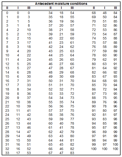
*Figure: Correlation between SCS Curve numbers and the antecedent moisture condition as given in /1/.

SCS Generalised Loss Model

Research has shown that it may be beneficial to apply another loss model than the standard SCS loss model. The SCS generalised loss model does not make use of the concept of an antecedent moisture content (AMC) but applies a general antecedent storage depth. This loss model in combination with the SCS unit hydrograph routing model complies completely with the TP108 approach often used in e.g. New Zealand and the United States.

Input data

Inputs that must be set for this loss model:

Initial abstraction depth [m] Curve number [-]

Loss computation

The SCS generalised loss model corresponds closely to the SCS standard loss model. However, it differs in a few important ways. The excess precipitation is still calculated by Equation the excess precipitation computed by the SCS Curve Number method:

\[ P_{e}~=~\frac{\left(P-I_{a}\right)^{2}}{P-I_{a}+S} \]

Equation: Excess precipitation from SCS generalised loss model using initial abstraction and retention.

but in this model the initial loss (initial abstraction depth) I_a is given directly as an input parameter.

The potential maximum retention S is calculated from a dimensionless curve number (CN) using the formula:

\[ S = \left(\left(\frac{1000}{CN}\right) - 10\right) \cdot 25.4 \cdot 10^{-3} \quad [m] \]

Equation: Potential maximum retention calculated from SCS curve number as a function of basin characteristics.

The curve number is an input parameter and is not changed during the simulation as for the SCS standard loss model.

Unit hydrograph routing model

Basic assumptions

The unit hydrograph method is a simple linear model that can be used to derive the hydrograph resulting from any amount of excess precipitation.

The unit hydrograph is a unit pulse response function of a linear hydrological system, i.e. the direct runoff hydrograph resulting from one unit of excess precipitation with the duration t_r.

The following basic assumptions are inherent in this model:

• Excess precipitation has a constant intensity within the effective duration,
• Excess precipitation is uniformly distributed over the whole catchment area.
• The base time of the direct runoff hydrograph resul¬ting from an excess precipitation with a given duration is constant.
• The ordinates of all direct runoff hydrographs of a common base time are directly proportional to the total amount of excess precipitation represented by each hydrograph.
• The principle of superposition applies to hydrographs resulting from continuous and/or isolated periods of uniform-intensity excess precipitation, as illustrated in the principle of superposition applied to hydrographs.
• For a given catchment, the hydrograph resulting from a given excess precipitation reflects the unchanging conditions of the catchment.

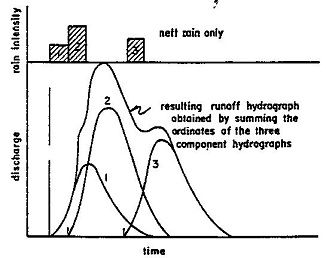
Figure: Principle of superposition applied to hydrographs.

Under natural conditions, the above assumptions cannot be perfectly met. However, in many cases the hydrological conditions come close enough to the above assumptions to generate satisfactory results. A more detailed discussion of the above assumptions can be found in /2/.

Principle of Calculation

In accordance with the principle of superposition, for each calculation time step the model determines the hydrograph corresponding to the excess rainfall, as generated by the loss model during this time step, and adds the response to the flow contributions generated in previous time steps.

Unit hydrograph models

SCS Unit Hydrographs

A unit hydrograph can be characterised by the duration of the unit rainfall t_r, resulting in the hydrograph and the lag time t_l, defined as the time difference between the centre of the unit rainfall event and the runoff peak.

From these two characteristics, the time to peak T_p, i.e. the time from the beginning of the storm event until the occurrence of peak runoff can be calculated as:

\[ T_p = \frac{t_r}{2} + t_l \]

Equation: Time to peak of unit hydrograph as sum of rainfall duration and basin lag time.

In reality, the unit hydrograph of a given catchment is unique. However, large efforts have been put into the development of synthetic unit hydrographs which are more or less generally applicable. Two such hydrographs are pre-specified in the model (see the SCS Synthetic Hydrographs: (a) Dimensionless hydrograph):

• SCS triangular unit hydrograph
• SCS dimensionless hydrographs

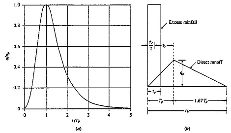
Figure: SCS Synthetic Hydrographs: (a) Dimensionless hydrograph;. (b) Triangular hydrograph

The user must specify the lag time to be used in a given calculation. The program will then scale the applied hydrograph accordingly, ensuring that the area under the curve equals to unity.

There are two ways of specifying the lag time:

• User defined value.
• Calculated from catchment characteristics using the standard SCS formula:

\[ t_{i}=(L\cdot3.28\cdot~10^{3})^{0.8}\cdot\frac{(~1000/~C N-9)^{0.7}}{(~1900\cdot Y^{0.5})} \]

Equation: SCS lag time formula for time to peak in unit hydrograph calculation.

Where:

Table: Variables in the SCS lag time calculation formula.

tl	Lag time in hours
L	Hydraulic length of the catchment in km
CN	The SCS curve number
Y	The average catchment slope in per cent

A unit-hydrograph derived from a time-area curve is considered as catchment-specific. Consequently, specification of arbitrary lag times are not allowed if the time-area method is applied. The program will simply use the lag time implicitly given by the time-area curve.

The time-area method in the UHM-model performs a pure trans¬lation of the excess precipitation hydrograph via the drainage network described using the channel travel time. This results in an outflow hydrograph, which ignores catchment storage effects.

Snyder Unit Hydrograph (SUH)

Standard SUH

From an analysis of ungaged watersheds varying in size from 30 to 30,000 km² in the Appalachian Highlands in the United States, Snyder published a description of a standard and required synthetic unit hydrographs in 1938. He published a relationship for estimating the unit hydrograph parameters from watershed characteristics. The relationship is shown in the snyder's Synthetic Unit Hydrograph.

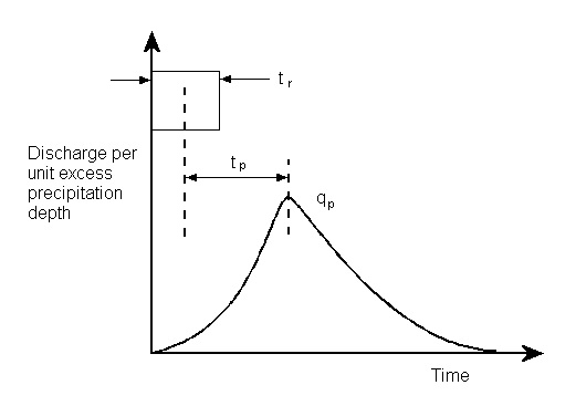
Figure: Snyder's Synthetic Unit Hydrograph.

For the standard unit hydrograph, Snyder defined the basin lag time t_p in hours to be related to the rainfall duration t_r in hours as follows:

\[ t_{p}~=~5.5~t_{r} \]

Equation: Basin lag time relation to rainfall duration in Snyder synthetic unit hydrograph.

For the required unit hydrograph, Snyder defined the basin lag time to be related to the watershed characteristics as follows:

\[ t_{\rho}~=~C_{1}C_{\ell}(L L_{c})^{0.3} \]

Equation: Snyder's basin lag time relating watershed characteristics to unit hydrograph timing.

Where:

Table: Variables in the Snyder basin lag time equation.

tp	Lag time in hours
C1	Conversion constant of 0.75
Ct	Watershed coefficient
L	Length of main stream from the outlet to the divide in km
Lc	Length of main stream from the outlet to a point nearest watershed centroid in km

The peak discharge per unit drainage area is found with the following relationship:

\[ q_{p}~=~\frac{C_{2}C_{p}}{t_{p}} \]

Equation: Peak discharge per unit drainage area from unit hydrograph theory.

Where:

Table: Variables in the peak discharge per unit drainage area equation.

qp	Peak discharge per unit drainage area in m3 per sec km2
C2	Conversion constant of 2.75
Cp	Peaking coefficient
tp	Lag time in hours

If the duration of the required unit hydrograph is significantly different from that specified by Equation the time to peak of unit hydrograph as sum of rainfall duration and basin lag time the following relationship could be used to relate the effective rainfall t_R in hours to the lag time t_pR in hours and peak discharge q_pR per unit area in m³ per sec km².

\[ t_{p R}=t_{p}-\frac{t_{r}-t_{R}}{4} \]

Equation: Adjusted peak rainfall duration for unit hydrograph related to required duration.

\[ q_{p R}~=~\frac{q_{p}t_{p}}{t_{p R}} \]

Equation: Unit hydrograph peak discharge scaled by rainfall duration and peak time ratio.

The base time of the hydrograph tb in hours can be found using the following relationship between peak discharge q_pR and the conversion constant C³ which equals 5.56:

\[ t_b = \frac{C_3}{q_p R} \]

Equation: Base time of unit hydrograph as a function of peak discharge and conversion constant.

The width W in hours of the unit hydrograph at a discharge equal to a certain percent of the peak discharge q_pR can be calculated using the following equation:

\[ W~=~C_{w}q_{p R}^{~-1.08} \]

Equation: Width of unit hydrograph at a specified percentage of peak discharge.

Where:

Table: Unit hydrograph width calculation coefficients.

Cw	1.22 for the 75 percent width and 2.14 for the 50 percent width

Alameda SUH

As part of a watershed study program completed in 1994, Alameda County, California developed site-specific equations to be used in conjunction with the Snyder unit hydrograph. The site-specific equations are documented in the September 1994 Hydrologic Modeling Evaluation Summary Report for Alameda County, California prepared by Alameda County Public Works Agency. There are two SUH equations that were modified as part of the Alameda County watershed study program. The first equation replaces the basin lag t_pR and the second equation replaces peaking factor C_p. The site specific equations should be used with caution outside of Alameda County, California.

\(t_{pR} = K n \left[\frac{L L_c}{\sqrt{S}}\right]^{-0.38}\)

\[ K = \begin{cases} 24 & \text{for } L > 1.7 \text{ miles} \\[1.5ex] 15.22 + 2.1464 L + \dfrac{8.6981}{L} & \text{for } L < 1.7 \text{ miles} \end{cases} \]

Equation: Storage coefficient K used in the Snyder unit hydrograph method.

Where:

Table: Variables in the Alameda County lag time equation.

tpR	Lag time in hours
K	Watershed coefficient
n	watershed factor specific to Alameda County, California
L	Length of main stream from the outlet to the divide in km
Lc	Length of main stream from the outlet to a point nearest watershed centroid in km
S	Average stream slope in ft per mile
Note	If K > 40 then K = 40

\[ C_p = 0.6 e^{0.06(S_o / A)} \]

Equation: Peaking coefficient as function of stream slope and basin area.

Where:

Table: Variables in the peaking coefficient equation.

Cp	Peaking coefficient (Cp = 0.85 if Cp from Equation the width of unit hydrograph at a specified percentage of peak discharge is greater than 0.85)
So	Average overland slope in percent (S > 5%)
A	Drainage area in square miles (for drainage area less than 5 square miles use 5)
Note	When overland slope < 5%, Cp = 0.6

User defined Hydrograph

River (MIKE 11 / MIKE HYDRO)

MIKE 1D engine also accepts user defined hydrograph (only available from MIKE 11 interface).

The user must specify the dimensionless flow in a time series with “Dimensionless factor” type. The calendar of the time series must be Relative temporal axis.

Calculation Time Step

If the SCS hydrographs are used, SCS suggests the calculation time step to be selected as 22% of the lag time and that it should not exceed 27% of the lag time.