Morphological updating

The morphological changes during a simulation are calculated separately for each sediment fraction in the form of local mass changes in each cross-section. Those changes are calculated by separate means for bed-load and suspended load.

Bed-load

For the bed-load, the mass changes are calculated using the Exner equation, i.e.:

\[ \frac{\Delta m_{1,i}}{\Delta t} = \rho s_{i}\ \left( Q_{b,in,i} - Q_{b,out,i} \right) \]

Equation: Exner equation for the bed-load mass change in a cross-section.

Where \(m_{1,i}\) [g/m²] denotes the sediment mass in the active layer of the considered fraction (\(i\)) per surface area in the cross-section, and \(Q_{b,i}\) are the volumetric sediment transport rates [m³/s] in and out of the cross-section.

A very simple numerical scheme is used for the calculation, in which the time-derivative is simply forward in time and the advective term can be calculated directly upstream and downstream of each cross-section due to the staggered grid adopted in MIKE 1D. In order to ensure a stable solution, the bed-load calculations adopt upwind flow areas when calculating the flow velocities used for the shear stress. This is done to prevent wiggles in the solution.

Suspended load

For the suspended load, we cannot use the Exner equation due to the accumulation of sediment in the water column (especially for fine sediment). Instead we use the source/sink terms in the advection-dispersion equation directly:

\[ \frac{\Delta m_{1,i}}{\Delta t} = D_{i} - E_{i} \]

Equation: Mass change from suspended load, taken from the deposition and erosion terms.

The (for each fraction) erosion (\(E_{i}\)) and deposition (\(D_{i}\)) denote the fluxes of sediment between the water and bed per surface area per time [g/m²/s].

Layer model

The layer model has three different modes.

0-layer

This choice is only available when simulating one single non-cohesive sediment component and corresponds to unlimited availability of sediment.

1-layer

Limited availability of sediment. The initial layer thickness is given directly as input or initialized as the difference between the initial bottom level and non-scouring bed level. A 1-layer model is always numerically valid, but physically it works best in situations with very thin sediment layers transported over fixed surfaces, e.g. sediment transport in pipes.

2-layer

Limited availability of sediment. Active and passive layer with interaction between the layers. A 2-layer model requires at least two sediment fractions in order to be selectable.

When using a 2-layer model, an extra step enters into the calculation loop. The step is performed after updating the passive layer (layer-1), which will deviate from the active layer thickness (target thickness) when it is updated. The two layers are now updated in an attempt to keep layer-1 equal to the target thickness. The thicknesses equivalent to the masses in the bed layers (\(j = 1\)-\(2\)) are first calculated:

\[ \Delta_{j} = \sum_{i}\frac{m_{j,i}}{s_{i} \cdot \rho \cdot (1 - n_{i})} \]

Equation: Layer thickness equivalent to the sediment masses stored in that layer.

The change in the interface between layer-1 and layer-2 can now be calculated:

\[ \Delta z = \Delta_{1} - \Delta_{a} \]

Equation: Change in the elevation of the interface between the active and passive layer.

Where:

• \(\Delta z\) — change in interface elevation
• \(\Delta_{1}\) — thickness of layer-1
• \(\Delta_{a}\) — active layer thickness (model parameter)

The highest theoretical value for \(\Delta z\) is \(\Delta_{1}\), which happens if the active layer thickness is zero. Although not possible to set the active layer thickness to zero, it can be set very low. In this case all the sediment in layer-1 should move to layer-2.

The minimum value of \(\Delta z\) is \(-\Delta_{a}\), which occurs when layer-1 is depleted (empty) during the time-step. In this case the interface should move down with a level change equal to the active layer thickness to get layer-1 to a thickness equal to the active layer thickness. However, this is not always possible because the thickness of layer-2 needs to be taken into consideration as well, such that the interface cannot move down more than the thickness of layer-2, i.e. combined with the upper limit we find:

\[ -\Delta_{2} \leq \Delta z \leq \Delta_{1} \]

Equation: Limits on the interface change, bounded by the thickness of each layer.

What this states is simply that the interface cannot move further down than the bottom of layer-2.

Having now established the interface change between layer-1 and layer-2, it is time to calculate the associated sediment exchange.

First consider the case where \(\Delta z\) is positive. In this case \(\Delta z\) will move from layer-1 to layer-2 with the bed composition of layer-1. This we can write as:

\[ m_{1,i} \leftarrow m_{1,i} - m_{1,i}\ \frac{\Delta z}{\Delta_{1}} = m_{1,i}\ \left( 1 - \frac{\Delta z}{\Delta_{1}} \right) \]

Equation: Updated layer-1 mass where the interface moves up.

\[ m_{2,i} \leftarrow m_{2,i} + m_{1,i}\ \frac{\Delta z}{\Delta_{1}} \]

Equation: Updated layer-2 mass where the interface moves up.

When looking at this we see that the sediment mass in layer-1 is scaled down with the same relative reduction for all sediment fractions, i.e. the relative distribution in layer-1 does not change, while the relative fraction composition in layer-2 will change.

The case where the interface moves down (\(\Delta z\) negative) means that the fraction \(\Delta z/\Delta_{2}\) of layer-2 will move to layer-1, i.e.:

\[ m_{1,i} \leftarrow m_{1,i} - m_{2,i}\ \frac{\Delta z}{\Delta_{2}} \]

Equation: Updated layer-1 mass where the interface moves down.

\[ m_{2,i} \leftarrow m_{2,i} + m_{2,i}\ \frac{\Delta z}{\Delta_{2}} = m_{2,i}\ \left( 1 + \frac{\Delta z}{\Delta_{2}} \right) \]

Equation: Updated layer-2 mass where the interface moves down.

Here the situation is reversed, such that the layer-2 masses are scaled with the same factor, i.e. no change in the layer-2 composition, while the layer-1 composition changes because layer-1 receives sediment from layer-2.

One notices that the range for \(\Delta z\) ensures in a very logical way here that each layer cannot be more than emptied.

Non-scouring bed level

Level below which there is no available sediment. Bottom level cannot come below this level.

Where both an initial layer depth and a non-scouring bed level is defined, the bottom level for the sediments is the largest of the two, i.e. the non-scouring bed level will only have an effect if it protrudes the initial layer depth level.

Cross section updating

The cross sections can be updated with three different methods.

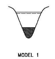
Figure: Cross section updating with Model 1, where sediment settles with a horizontal surface.

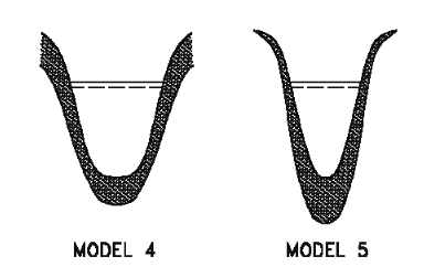
Figure: Cross section updating with Model 4 and Model 5, where sediment settles over the whole section or preferentially in the bottom.

Model 1

Sediment settles with a horizontal surface independently of cross section beneath sediment level. This method is usually used for pipes and other cross sections with a fixed, hard bottom level, typically made of concrete or plastic.

Model 4

Sediment settles equally over the entire cross sections. As a result, the cross section is not changed but simply moved up and down when the sediment erodes or deposits.

Model 5

Sediments settles more in bottom of cross section. The deposition is scaled with the depth of the cross section below the flood plain level. The flood plain level is by default the top of the cross section but can be user specified or set to be the smallest of the low flow bank markers. When cross section is almost fully filled up to the flood plain level, Model 4 is applied for any further deposition.