NAM Rainfall Runoff Model

NAM Rainfall Runoff Model

Introduction

The NAM hydrological model simulates the rainfall-runoff processes occurring at the catchment scale. NAM forms part of the rainfall-runoff (RR) module of the 1D river modelling system. The rainfall-runoff module can either be applied independently or used to represent one or more contributing catchments that generate lateral inflows to a river network. In this manner it is possible to treat a single catchment or a large river basin containing numerous catchments and a complex network of rivers and channels within the same modelling framework.

NAM is the abbreviation of the Danish “Nedbør-Afstrømnings-Model”, meaning precipitation-runoff-model, also named RDII in English standing for Rainfall Dependent Inflow and Infiltration model. This model was originally developed by the Department of Hydrodynamics and Water Resources at the Technical University of Denmark ¹⁰.

A mathematical hydrological model like NAM is a set of linked mathematical statements describing, in a simplified quantitative form, the behaviour of the land phase of the hydrological cycle. NAM represents various components of the rainfall-runoff process by continuously accounting for the water content in four different and mutually interrelated storages. Each storage represents different physical elements of the catchment. NAM can be used either for continuous hydrological modelling over a range of flows or for simulating single events.

The NAM model can be characterised as a deterministic, lumped, conceptual model with moderate input data requirements. A description of the classification of hydrological models is given in Abbott and Refsgaard (1996) ¹. Refsgaard and Knudsen (1997) ¹² compare a number of different types of hydrological model, including the NAM model, in terms of both data requirements and model performance.

The NAM model is a well-proven engineering tool that has been applied to a number of catchments around the world, representing many different hydrological regimes and climatic conditions.

Introduction

The NAM hydrological model simulates the rainfall-runoff processes occurring at the catchment scale. NAM forms part of the rainfall-runoff (RR) module of the 1D river modelling system. The rainfall-runoff module can either be applied independently or used to represent one or more contributing catchments that generate lateral inflows to a river network. In this manner it is possible to treat a single catchment or a large river basin containing numerous catchments and a complex network of rivers and channels within the same modelling framework.

NAM is the abbreviation of the Danish “Nedbør-Afstrømnings-Model”, meaning precipitation-runoff-model, also named RDII in English standing for Rainfall Dependent Inflow and Infiltration model. This model was originally developed by the Department of Hydrodynamics and Water Resources at the Technical University of Denmark ¹⁰.

A mathematical hydrological model like NAM is a set of linked mathematical statements describing, in a simplified quantitative form, the behaviour of the land phase of the hydrological cycle. NAM represents various components of the rainfall-runoff process by continuously accounting for the water content in four different and mutually interrelated storages. Each storage represents different physical elements of the catchment. NAM can be used either for continuous hydrological modelling over a range of flows or for simulating single events.

The NAM model can be characterised as a deterministic, lumped, conceptual model with moderate input data requirements. A description of the classification of hydrological models is given in Abbott and Refsgaard (1996) ¹. Refsgaard and Knudsen (1997) ¹² compare a number of different types of hydrological model, including the NAM model, in terms of both data requirements and model performance.

The NAM model is a well-proven engineering tool that has been applied to a number of catchments around the world, representing many different hydrological regimes and climatic conditions.

Model structure

A conceptual model like NAM is based on physical structures and equations used together with semi-empirical ones. Being a lumped model, NAM treats each catchment as a single unit. The parameters and variables represent, therefore, average values for the entire catchment. As a result some of the model parameters can be evaluated from physical catchment data, but the final parameter estimation must be performed by calibration against time series of hydrological observations.

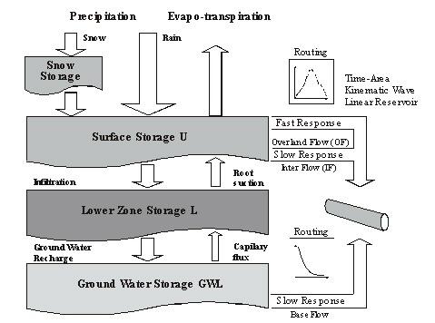
Figure: Model structure of the NAM.

The model structure is shown in the model structure of the NAM. It is an imitation of the land phase of the hydrological cycle. NAM simulates the rainfall-runoff process by continuously accounting for the water content in four different and mutually interrelated storages that represent different physical elements of the catchment. These storages are:

• Snow storage
• Surface storage
• Lower or root zone storage
• Groundwater storage

In addition NAM allows treatment of man-made interventions in the hydrological cycle such as irrigation and groundwater pumping.

Based on the meteorological input data NAM produces catchment runoff as well as information about other elements of the land phase of the hydrological cycle, such as the temporal variation of the evapotranspiration, soil moisture content, groundwater recharge, and groundwater levels. The resulting catchment runoff is split conceptually into overland flow, interflow and baseflow components.

The rainfall passing through the snow storage is controlled by the temperature conditions and the current amount of snow on the catchment surface.

Moisture interception on the vegetation, as well as water trapped in depressions and in the upper-most cultivated part of the ground is represented as surface storage.

Moisture in the root zone, a ground layer below ground surface from where the vegetation can draw water for transpiration, is described as a storage in the lower ground zone, i.e. root zone storage.

The amount of water in the surface storage is continuously diminished by evapo-transpirative consumption set as potential evapo-transpiration, as well as by horizontal leakage (interflow) in the upper ground level. In situations when there is a maximum surface storage achieved, some of the excess water will enter the streams as overland flow, whereas the remainder is diverted as infiltration into the lower zone and further as percolation into the groundwater storage.

Moisture in the lower zone is subject to consumptive loss from evapo-transpiration. This process starts when the surface storage is completely exhausted, and in that situation the actual evaporation depends on the relative contents of the moisture in the lower zone. Additionally, the amount of moisture in the lower zone influences the process of overland flow and amount of water that enters the groundwater storage as recharge.

Data requirement

The basic input requirements for the NAM model consist of:

• Model parameters
• Initial conditions
• Meteorological data
• Streamflow data for model calibration and validation

The basic meteorological data requirements are:

• Rainfall
• Potential evapotranspiration

In the case of snow modelling the additional meteorological data requirements are:

• Temperature
• Radiation (optional)

The NAM model also allows modelling of man-made interventions in the hydrological cycle in terms of irrigation and groundwater pumping. In this case time series of irrigation and groundwater abstraction rates are required.

In this section the meteorological and hydrological data are described. The model parameters and initial conditions are described in the subsequent sections.

Meteorological data

Rainfall

Urban (MIKE+)

Rainfall data are specified either as depth or as intensity (the latter is only available from the MIKE+ interface).

The time resolution of the rainfall input depends on the objective of the study and on the time scale of the catchment response. In many cases daily rainfall values are sufficient, but in rapidly responding catchments where accurate representation of the peak flows is required, rainfall input on a finer resolution may be required.

For validation process, resolution of the rainfall time series should correspond to the time resolution of measured discharges, e.g. daily average discharges.

Rainfall data with any (variable) time increments can be specified in the rainfall input. The NAM model will then make the necessary interpolations according to the simulation time step.

Potential evapotranspiration

The evapotranspiration is a physical process where water is transformed into vapor. Real evaporation or, more correctly, the actual evaporation includes evaporation from snow and ground surfaces of all types, interception from vegetation and its transpiration.

Interception is a part of rainfall that never reaches the ground but adheres to the vegetation and thereafter evaporates. Transpiration is water evaporation from inner surfaces in the plants, leaves and needles.

Urban (MIKE+)

The evapotranspiration specified in NAM model is the potential evaporation i.e. possible evaporation as a depth or intensity (the latter is only available from the MIKE+ interface).

When daily time steps are used, monthly values of potential evapotranspiration are usually sufficient. In this case only minor improvements can be obtained by specifying daily values instead of monthly values. For small time steps, however, the diurnal variation of the evapotranspiration may be important.

Temperature

Temperature data are required if snow accumulation and melt are included in the simulations. The temperature is specified in degree Celsius (°C).

The resolution in time for the temperature especially concerns areas where the snow melting process is of great importance. During the snow season, the time increments in the temperature data should reflect the length of the time step in the simulation, e.g. daily mean temperatures.

The temperature data at a given time represents the average temperature since the last entered data.

Radiation

River (MIKE 11 / MIKE HYDRO)

Actual incoming short wave radiation data can optionally be used as input in the extended snow module. The radiation data are specified in W/m². The value at a given time represents the average radiation since the last entered data.

Mean area weighting

River (MIKE 11 / MIKE HYDRO)

The NAM model simulates the rainfall-runoff process in a lumped fashion so provision is given for combining meteorological data from different stations within a single catchment or sub-catchment into a single time series of weighted averages. The resulting time series will represent the mean area values of rainfall and potential evapotranspiration for a catchment.

The weights are user-defined and can be determined based e.g. on the Thiessen method. In the case of missing values the weighting procedure will redistribute the weights appropriately. Therefore, it is not necessary to specify weight combinations for all possible combinations of missing stations. Alternatively, the user can explicitly specify the weights when data are missing from one or more stations. A weight of “-1” is given to non-reporting stations, indicating missing data.

When rainfall data are available from stations with different reporting frequency, e.g. both daily and hourly stations, then the distribution in time of the average catchment rainfall may be determined using a weighted average of the high-frequency stations. It is possible to use all stations to determine the daily mean rainfall over the catchment and subsequently use the hourly stations to distribute this daily rainfall in time. Different weight combinations for different cases of missing values may be applied also to the calculation of the distribution in time.

Hydrological data

Discharge

River (MIKE 11 / MIKE HYDRO)

Observed discharge data at the catchment outlet are required for comparison with the simulated runoff for model calibration and validation, they are specified as discharge (e.g. m³/s). The discharge data at any particular time is the average discharge since the last entered data.

Irrigation

River (MIKE 11 / MIKE HYDRO)

If the irrigation module is included in the NAM simulation, an additional rainfall time series is required to provide information on the amount of irrigation water. The data are specified as depth.

Groundwater abstraction

River (MIKE 11 / MIKE HYDRO)

When the effect of groundwater abstraction is expected to have a significant effect on the overall groundwater levels or catchment baseflow, pumping rates can be specified to account for these withdrawals. The groundwater abstraction data are treated as accumulated totals where the abstraction associated with any particular time is the abstraction since the last entered value. The data are specified as depth.

Basic modelling components

The implemented conceptualisation of the physical processes treated by NAM model is illustrated in the model structure of the NAM and exposed below in full detail.

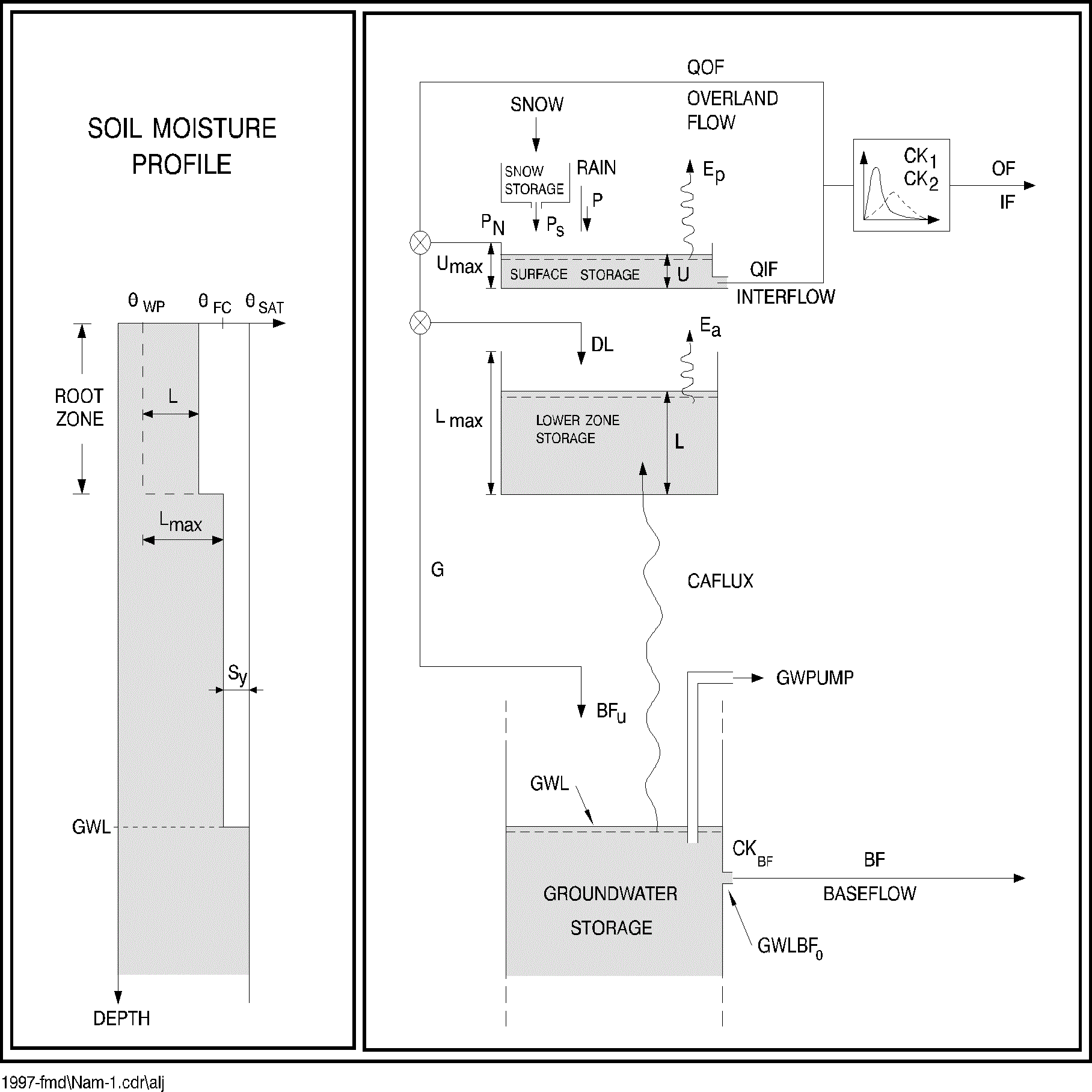
Figure: Conceptual model of NAM.

Surface storage

Moisture intercepted on the vegetation as well as water trapped in depressions and in the uppermost, cultivated part of the ground is represented as surface storage. U_max denotes the upper limit of the amount of water in the surface storage.

The amount of water, U, in the surface storage is continuously diminished by evaporative consumption as well as by horizontal leakage (interflow).

When the surface storage spills, i.e. when U > U_max, some of the excess water, P_N, will enter the streams as overland flow, whereas the remainder is diverted as infiltration into the lower zone and groundwater storage.

Lower zone or root zone storage

The soil moisture in the root zone, a soil layer below the surface from which the vegetation can draw water for transpiration, is represented as lower zone storage. L~max ~denotes the upper limit of the amount of water in this storage.

Moisture in the lower zone storage is subject to consumptive loss from transpiration. The moisture content controls the amount of water that enters the groundwater storage as recharge and the interflow and overland flow components.

Evapotranspiration

Evapotranspiration demands are initially met at the potential rate from the surface storage. If the moisture content U in the surface storage is less than these requirements (U < E_p), the remaining fraction is assumed to be withdrawn by root activity from the lower zone storage at an actual rate E_a. E_a is proportional to the potential evapotranspiration and varies linearly with the relative soil moisture content, L/L_max, of the lower zone storage

\[ E_a = (E_p - U) \frac{L}{L_{max}} \]

Equation: Actual evapotranspiration from lower zone storage proportional to soil moisture content.

Overland flow

When the surface storage spills, i.e. when U > U_max, the excess water P_N gives rise to overland flow as well as to infiltration. QOF denotes the part of P_N that contributes to overland flow. It is assumed to be proportional to P~N ~and to vary linearly with the relative soil moisture content, L/L_max, of the lower zone storage

\[ QOF = \begin{cases} CQOF\dfrac{L/L_{max} - TOF}{1 - TOF}P_{N} & \text{for } L/L_{max} > TOF \\[1.5ex] 0 & \text{for } L/L_{max} \leq TOF \end{cases} \]

Equation: Overland flow as a function of the relative moisture content of the root zone storage.

Where:

Table: Parameters for overland flow calculation.

CQOF	Overland flow runoff coefficient (0 £ CQOF £ 1)
TOF	Threshold value for overland flow (0 £ TOF £ 1)

The proportion of the excess water P_N that does not run off as overland flow infiltrates into the lower zone storage. A portion, DL, of the water available for infiltration, (P_N -QOF), is assumed to increase the moisture content L in the lower zone storage. The remaining amount of infiltrating moisture, G, is assumed to percolate deeper and recharge the groundwater storage.

Interflow

The interflow contribution, QIF, is assumed to be proportional to U and to vary linearly with the relative moisture content of the lower zone storage.

\[ QIF = \begin{cases} \left(CKIF\right)^{-1}\dfrac{L/L_{max} - TIF}{1 - TIF}U & \text{for } L/L_{max} > TIF \\[1.5ex] 0 & \text{for } L/L_{max} \leq TIF \end{cases} \]

Equation: Interflow as a function of the relative moisture content of the root zone storage.

Where:

Table: Parameters for interflow calculation.

CKIF	Time constant for interflow
TIF	Root zone threshold value for interflow (0 £ TIF £ 1)

Interflow and overland flow routing

The interflow is routed through two linear reservoirs in series with the same time constant CK₁₂. The overland flow routing is also based on the linear reservoir concept but with a variable time constant

\[ \begin{array}{r}{C K=\left\{\begin{array}{l l}{C K_{12}}&{\mathrm{for}~O F<O F_{m i n}}\\ {C K_{12}\!\!\left(\frac{O F}{O F_{m i n}}\right)^{-\beta}~\mathrm{for}~O F\geq O F_{m i n}}\end{array}\right.}\end{array} \]

Equation: Variable time constant for overland flow routing dependent on overland flow magnitude.

Where:

Table: Parameters for overland flow routing calculations.

OF	Overland flow intensity (mm/hour)
OFmin	Upper limit for linear routing (= 0.4 mm/hour),
b	= 0.4

The constant b = 0.4 corresponds to using the Manning formula for modelling the overland flow. Equation the variable time constant for overland flow routing dependent on overland flow ensures in practice that the routing of real surface flow is kinematic, while subsurface flow being interpreted by NAM as overland flow (in catchments with no real surface flow component) is routed as a linear reservoir.

Urban (MIKE+)

The reservoir time constants CK₁ and CK₂ taken equal to CKOF in both reservoirs.

Groundwater recharge

The proportion of net excess rainfall, Pn, that does not run off as overland flow infiltrates into the lower zone storage representing the root zone. A portion, DL, of the amount of infiltration, (Pn-OF), is assumed to increase the moisture content, L, in the lower zone storage. The remaining amount of infiltrating water, G, is assumed to percolate deeper and recharge the groundwater storage. The G and DL are calculated from:

\[ G = \begin{cases} \left(P_{N} - QOF\right)\dfrac{L/L_{max} - TG}{1 - TG} & \text{for } L/L_{max} > TG \\[1.5ex] 0 & \text{for } L/L_{max} \leq TG \end{cases} \]

Equation: Groundwater recharge as a function of the relative moisture content of the root zone storage.

and

\(\Delta L = P_N - QOF - G\) 

Where:

Table: Threshold value for groundwater recharge.

TG	Root zone threshold value for groundwater recharge (0 £ TG £ 1)
TG	Root zone threshold value for groundwater recharge (0 £ TG £ 1)

Baseflow

The baseflow BF from the groundwater storage is calculated as the outflow from a linear reservoir with time constant CK_BF.

Extended groundwater components

Drainage to or from neighbouring catchments

Local geological conditions may cause part of the infiltrating water to drain to neighbouring catchments. In NAM this loss of water can be described by specifying the ratio of the groundwater catchment area to the topographical catchment area, C_area, with a value less than one. In this case the proportion (1-C_area) of the recharge G is drained to neighbouring catchments. Similarly, water may be drained from neighbouring catchments, implying an increased groundwater recharge in the catchment (C_area > 1).

Lower groundwater storage

For a better description of the baseflow, an additional (lower) groundwater storage can be defined. In this case the upper groundwater storage provides the fast responding component of the baseflow, whereas the lower storage usually has a slower response. The recharge to the lower storage is given as a proportion CQ_LOW of the total recharge G. The routing from the lower storage is described by a linear reservoir with time constant CK_LOW.

Shallow groundwater reservoir description

The groundwater level is calculated from a continuity consideration accounting for recharge G, capillary flux CAFLUX, net groundwater abstraction GWPUMP, and baseflow BF. The inclusion of capillary flux and groundwater pumping are optional. The groundwater storage can be treated in two different ways, either as a simple linear reservoir as described in Section  Baseflow (p. 175) or as a shallow groundwater reservoir.

The shallow groundwater reservoir description is appropriate for lowland catchments with little topographical variation and the potential for water logging. The baseflow is given by

\[ BF = \begin{cases} \left(GWL_{BF0} - GWL\right)S_{Y}\left(CK_{BF}\right)^{-1} & \text{for } GWL \leq GWL_{BF0} \\[1.5ex] 0 & \text{for } GWL > GWL_{BF0} \end{cases} \]

Equation: Baseflow as a function of the groundwater level.

Where:

Table: Parameters for baseflow calculation with shallow groundwater reservoir.

SY	Specific yield of the reservoir
GWL	Groundwater table depth
GWLBF0	Maximum groundwater table depth, which causes baseflow

The parameter GWL_BF0 can be interpreted as the distance between the average ground level of the catchment to the water level of the river. Due to the variation in the river water level throughout the year GWL_BF0 can be given a significant annual variation.

Capillary flux

The capillary flux CAFLUX of water from the groundwater to the lower zone storage is assumed to depend on the depth of the groundwater table below the ground surface, GWL, as well as on the relative moisture content, L/L_max, of the lower zone storage

\[ CAFLUX = \sqrt{1 - L/L_{max}}\left( \frac{GWL}{GWL_{FL1}} \right)^{-\alpha} \text{(mm/day)} \\[1ex] \alpha = 1.5 + 0.45 GWL_{FL1} \]

Equation: Capillary flux from the groundwater storage to the root zone storage.

Where:

Table: Groundwater table depth parameter for capillary flux calculation.

GWLFL1	Groundwater table depth at which the capillary flux is 1 mm/day when the lower zone storage is completely dry

Equation (7.7) provides a good fit to the theoretical relationship between the capillary flux, the depth to the water table and the soil moisture content proposed by Rijtema (1969) ¹³.

The process is activated if a value of GWL_FL1 different than zero is specified.

Snow module

Snow accumulation and melt are important hydrological processes in river basins where the snow pack acts as a storage in which precipitation is retained during the cold season and subsequently released as melt water during the warmer parts of the year.

The snow melt component of the runoff is incorporated as an integrated module within NAM. This component is optional and temperature data is only required if the snow routine is selected. Normally the precipitation enters directly into the surface storage. However, during cold periods precipitation is retained in the snow storage from which it is melted in warmer periods. Two different models can be applied; a simple lumped calculation or a more general approach that divides the catchment into a number of altitude zones with separate snow melt parameters, temperature and precipitation input for each zone.

Accumulation and melting of snow

Several investigations (e.g. ¹⁴) have shown that the shift between precipitation in the form of rain and snow usually takes place when the air temperature is within a narrow interval close to 0^ o^C. In the snow module it is assumed that the precipitation falls as rain when the air temperature is above a certain base temperature level, T₀, which can be specified by the user.

The snowmelt QS is calculated using a degree-day approach

\[ QS = \begin{cases} C_{snow}(T-T_0) & \text{for } T > T_0 \\ 0 & \text{for } T \leq T_0 \end{cases} \]

Equation: Snowmelt calculated using degree-day method proportional to temperature excess above melt threshold.

Where:

Table: Degree-day coefficient for snow melt.

Csnow i	Degree-day coefficient

The generated melt water is retained in the snow storage as liquid water until the total amount of liquid water exceeds the water retention capacity of the snow storage. The excess melt water P_S is routed to the NAM model where it contributes to the surface storage. The excess melt water contribution P_S to NAM is

\[ \begin{array}{r}{P_{\mathcal{S}}=\left\{\begin{array}{l l}{Q_{m e l t}~\mathrm{for}~W R\!\geq C_{w r}\mathcal{S}_{s n o w}}\\ {0\qquad\mathrm{for}~W R<C_{w r}\mathcal{S}_{s n o w}}\end{array}\right.}\end{array} \]

Equation: Excess melt water contribution to NAM model when snow water retention is exceeded.

Where:

Table: Parameters for water retention in snow storage.

WR	Water retention in the snow storage
Cwr	Water retention coefficient
Ssnow	Snow storage

Urban (MIKE+)

From MIKE+ interface, the Water retention coefficient C~wr ~is set to 8%.

The new snow storage is calculated by subtracting the excess melt water P_S from the snow storage.

The rain fraction is added as liquid water and is retained in the snow storage if the total liquid water content of the snow pack is below its water retaining capacity. When the air temperature is below T₀, the liquid water content in the snow storage freezes with rate C_snow. Evaporation from the snow pack is neglected.

Altitude-distributed snowmelt model

River (MIKE 11 / MIKE HYDRO)

This section is only available from MIKE 11 interface.

Introduction

In mountainous areas temperature, precipitation and snow cover often vary significantly within a single catchment. The runoff simulation for such areas can be improved by dividing the catchment into smaller zones and maintain individual snow storage calculations in each zone.

The altitude-distributed snow model calculates melt water in a number of altitude zones using the degree-day approach. Since in many cases the hydro-meteorological information from mountain basins is quite sparse, the module also includes facilities for distribution of the meteorological information with altitude.

Structure of the altitude-distributed snowmelt module

The snow melt module allows the user to define a number of altitude zones within a NAM catchment and adjust the snow melt parameters and the temperature and precipitation input to the model for each zone. The snow melt module maintains individual snow storages and calculates accumulation and melting of snow for each altitude zone. The simulated melt water from all zones is subsequently superposed and routed through the NAM model as illustrated in the structure of the NAM model with extended snow module. This implies that the same model parameters for infiltration, runoff and groundwater routing are applied for all altitude zones. Such an approach will be appropriate for the large majority of mountain catchments.

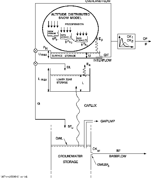
Figure: Structure of the NAM model with extended snow module.

In special cases where differentiation is needed also in the other parameters the catchment in question can be divided into two or more sub-catchments. The total simulated discharge is then found by accumulating the simulated discharge from the different sub-catchments using the combined catchment approach in the MIKE 11 RR editor.

In the altitude-distributed snow model, snow melting only takes place from the snow-covered part of each zone. When the water equivalent of the snow pack falls under a user-specified value (minimum storage for full coverage), the area coverage will be reduced linearly with the snow storage in the zone.

Snow will not necessarily melt on the location where it falls. Due to wind transport the snow accumulation at wind exposed sites may often be significantly smaller than at locations well sheltered against wind. Wind exposed conditions are often present at higher altitudes where vegetation is sparse and wind velocities generally high. Furthermore, for the higher parts of mountain ranges, steep slopes having a limited snow storage capacity will often dominate. Snow storage in excess of this capacity will at such locations generate avalanches which transport the snow to lower altitudes. Hence, some of the snow falling on wind exposed and/or steep highlands may not melt on the location but be deposited and melting at lower altitudes. To account for such re-distribution of snow and avoid unrealistic accumulation of snow in the cold upper zones a user specified upper limit of the snow storage in the individual zones has been introduced in the model. Snow storage exceeding this value will be transferred to the neighbouring lower zone.

Adjustment of temperature and precipitation to altitude zones

The altitude-distributed snow model operates with three meteorological reference time series; precipitation, temperature and potential evapotranspiration. In order to account for the large variations in precipitation and temperature with altitude the reference series can be adjusted for each altitude zone in two different ways:

• lapse rate corrections
• individual correction factors applied for each zone

The engine uses the individual factors for each zone. The lapse rate corrections are used to calculate the individual correction factors before starting the simulation.

Lapse rate corrections

The lapse rate correction approach is a very simple but powerful way of adjustment in which the temperature and the precipitation are assumed to vary linearly with the altitude. The only input data required are the average altitude of the various zones, a reference altitude of the time series, and the lapse rates. The temperature lapse rates, however, are known to be quite variable, ranging from high values under dry conditions to lower values under wet conditions. Hence, in the model it is possible to specify two different temperature lapse rates to be used during dry and wet weather conditions, respectively. The model applies the “wet” lapse rate during days with precipitation and the “dry” lapse rate during the rest of the time.

The temperature in each zone is adjusted by the following formula:

\[ T_{zone} = \begin{cases} T_{ref}+(H_{zone}-H_{ref})\beta_{dry} & \text{for } P=0 \\ T_{ref}+(H_{zone}-H_{ref})\beta_{wet} & \text{for } P>0 \end{cases} \]

Equation: Temperature lapse rate applied to different elevation zones with separate dry and wet rates.

Where:

Table: Temperature lapse rate parameters.

Tzone	Temperature in the considered zone
Tref	Temperature at the reference temperature station
Hzone	Average height in the zone
Href	Height at the reference temperature station
bdry	Temperature lapse rate for dry conditions
bwet	Temperature lapse rate for wet conditions

The precipitation in each altitude zone is calculated from the precipitation at the reference station:

\[ P_{z o n e}~=~P_{r e f}(~1+(H_{z o n e}~-~H_{r e f})\alpha) \]

Equation: Precipitation adjustment for altitude zone using linear lapse rate.

Where:

Table: Precipitation lapse rate parameters.

Pref	Precipitation at the reference precipitation station
Href	Height at the reference precipitation series
a	Precipitation lapse rate

Individual correction factors applied for each zone

In this case corrections have to be specified by the user for each altitude zone. This method requires more input but also offers a larger flexibility. The corrected meteorological series are calculated using the formulae:

\[ T_{zone} = \begin{cases} T_{ref}+T_{cor,zone,dry} & \text{for } P=0 \\ T_{ref}+T_{cor,zone,wet} & \text{for } P>0 \end{cases} \]

Equation: Temperature correction factors for altitude zones depending on precipitation occurrence.

\[ P_{zone} = P_{ref}\left(1 + P_{cor, zone}\right) \]

Equation: Altitude-corrected precipitation for a zone applied as a relative correction factor.

Where:

Table: Temperature and precipitation correction factors for altitude zones.

Tcor,zone,wet	Actual temperature corrections for wet conditions
Pcor,zone,dry	Actual temperature corrections for dry conditions,
Pcor,zone	Relative precipitation correction

If it is not possible to represent the meteorological conditions in the catchment by adjustment of one series only, the catchment may be divided into smaller sub-catchments in which one series will be representative. The discharges for the individual sub-catchments are then superposed using the combined catchment approach in the MIKE 11 RR editor.

Extended components

Seasonal variation of degree-day coefficient

River (MIKE 11 / MIKE HYDRO)

The simple degree-day approach for calculating snow melt described by equation the snowmelt calculated using degree-day method proportional to temperature excess can be extended by using a seasonal variation of the degree-day coefficient C_snow. This variation reflects in a conceptual way the seasonal variation of the incoming short wave radiation and the variation in the albedo of the snow surface during the snow season. The albedo is very high (about 0.8) for new, cold snow falling in the beginning of the accumulation season and then decreases with the age of the snow (to a minimum value of about 0.3 in the end of the season).

Radiation

River (MIKE 11 / MIKE HYDRO)

The melting effects caused by the absorbed short wave radiation can be explicitly modelled. In this case an additional snow melting is calculated as

\[ \Delta QS = C_{rad}R \]

Equation: Additional snow melt from absorbed short-wave radiation with radiation coefficient.

Where:

Table: Parameters for radiation effect on snow melt.

Crad	Radiation coefficient,
R	Incoming short wave radiation

The total amount of snow melt is calculated as the sum of the snow melt rates given by Equations the snowmelt calculated using degree-day method proportional to temperature excess, the additional snow melt from absorbed short-wave radiation with radiation, and the additional snowmelt from condensation of humid air and advective heat from (optional), respectively.

Condensation of humid air and heat contribution from rainfall

River (MIKE 11 / MIKE HYDRO)

The melting effects from condensation of humid air on the snow surface and the advective heat transferred to the snow pack by precipitation can be explicitly modelled. The effects are calculated as an additional snowmelt

\[ \Delta QS = C_{rain}P(T - T_0) \]

Equation: Additional snowmelt from condensation of humid air and advective heat from rainfall using degree-day method.

Where:

Table: Parameters for rainfall effect on snow melt.

Crain	Degree-day coefficient,
P	Rainfall

The total amount of snow melt is calculated as the sum of the snow melt rates given by the snowmelt calculated using degree-day method proportional to temperature excess, the additional snow melt from absorbed short-wave radiation with radiation (optional), and the additional snowmelt from condensation of humid air and advective heat from, respectively.

Irrigation module

River (MIKE 11 / MIKE HYDRO)

This section concerns the irrigation module, which is only available from MIKE 11 interface.

Introduction

Minor irrigation schemes within a catchment will normally have negligible influence on the catchment hydrology, unless transfer of water over catchment boundaries is involved. Large schemes, however, may significantly affect the runoff and the groundwater recharge through local increases in evapotranspiration and infiltration as well as through operational and field losses.

The irrigation module of NAM may be applied to describe the effect of irrigation on the following aspects:

• The overall water balance of the catchment. This will be affected mainly by the increased evapotranspiration and by possible external water sources for irrigation.
• Local infiltration and groundwater recharge in irrigated areas.
• The distribution of catchment runoff amongst different runoff components (overland flow, interflow, baseflow). This may be influenced by the increased infiltration in irrigated areas as well as by local abstraction of irrigation water from groundwater or streams.

For each irrigation area within the catchment a NAM sub-catchment is defined with individual model parameters. The non-irrigated areas are modelled by defining a general NAM sub-catchment. The total simulated discharge is then found by accumulating the simulated discharge from the different sub-catchments using the combined catchment approach in the MIKE 11 RR editor.

Structure of the irrigation module

The structure of the irrigation module is illustrated in the structure of the NAM irrigation module.

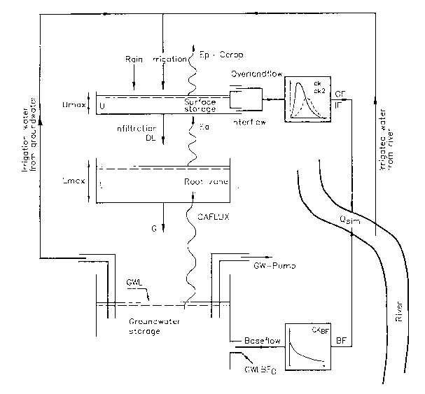
Figure: Structure of the NAM irrigation module.

Water supplied to the surface storage in irrigated areas will be a sum of precipitation P and irrigation water P_ir. The potential evapotranspiration may vary with crop type and the stage of growth. The irrigation module accounts for this by allowing the user to specify monthly varying crop coefficients C_crop for each irrigation area. The potential evapotranspiration for a specific crop is given by

\[ E_{p, crop} = C_{crop}E_{p} \]

Equation: Potential evapotranspiration adjusted for crop type through crop coefficient.

Where:

Table: Reference time series for potential evapotranspiration.

Ep	Reference time series of potential evapotranspiration

Infiltration I is taken directly from the surface storage to the lower zone and groundwater storages and is calculated as a function of the moisture content in the lower zone L

\[ I = \begin{cases} k0_{inf}L_{max}/L & \text{for } k0_{inf}L_{max}/L < U \\ U & \text{for } k0_{inf}L_{max}/L \geq U \end{cases} \]

Equation: Infiltration from surface storage as a function of moisture content in lower zone.

Where:

Table: Infiltration factor parameter describing infiltration rate.

k0inf	infiltration factor describing the infiltration rate at field capacity (i.e. L = Lmax)

A portion G of the infiltration is assumed to percolate deeper and recharge the groundwater storage. This portion is, as in the general NAM model, calculated as a function of the conditions in the lower zone storage

\[ G = \begin{cases} I\frac{L/L_{max}-TG}{1-TG} & \text{for } L/L_{max} > TG \\ 0 & \text{for } L/L_{max} \leq TG \end{cases} \]

Equation: Groundwater recharge as fraction of infiltration depending on lower zone saturation.

Where:

Table: Threshold value for groundwater recharge in irrigation module.

TG	root zone threshold value for groundwater recharge

The remaining part DL is assumed to increase the moisture content in the lower zone

\[ \Delta L = I -G \]

Equation: Lower zone moisture storage change from infiltration and groundwater discharge.

If the maximum surface storage U_max is exceeded, the general NAM model diverts the excess water into overland flow (QOF) and infiltration. In the irrigation module infiltration has been accounted for as described above, and hence the excess water is added directly to overland flow.

Irrigation water can be abstracted from three different sources. The amount of water taken from each source type is determined by specifying fixed percentages of P_ir for each source type:

• local groundwater (PC_lgw)
• local river (PC_lr)
• external river (PC_exr)

The term “local” means within the actual NAM catchment. If irrigation water is abstracted from local groundwater, it will be subtracted from the groundwater storage and the groundwater level will then be reduced with the amount

\[ \Delta G W L=\frac{\Delta t P C_{I g w}P_{i r}}{S_{Y}} \]

Equation: Groundwater level change due to irrigation abstraction from local groundwater storage.

Table: Parameters for groundwater level change calculation.

SY	Specific yield
Dt	Time step used in the calculations

Where:

If the water is abstracted from a local river, it will be subtracted from the calculated runoff

\[ \Delta Q_{sim} = \Delta tPC_{lr}P_{ir} \]

Equation: Simulated discharge change from water diverted for irrigation abstraction.

If the water is imported from a river outside the NAM catchment (external), no subtractions are made.

A part of the water diverted for irrigation will be lost on its way to the fields. The losses may include evaporation and seepage from channels, illegal off-takes, and operational losses (i.e. water that is diverted to the irrigation area but is not being utilised). In the irrigation module, the user may specify percentages of the irrigation water P_ir that is lost, i.e.

• evaporation losses (PC_evap)
• seepage losses (PC_gw)
• operational losses contributing to overland flow (PC_of)

The losses may vary in time on a monthly basis.

Due to the different losses the irrigation water is reduced with the amount

\[ \Delta P_{ir} = P_{ir}\left(PC_{evap} + PC_{gw} + PC_{of}\right) \]

Equation: Irrigation water reduction due to cumulative losses from evaporation, groundwater, and overland flow.

The operational losses yields an increase in the overland flow

\[ \Delta OF = \Delta tPC_{of}P_{ir} \]

Equation: Operational losses contribution to overland flow in irrigation systems.

The seepage losses contributes to an increase in the groundwater level

\[ \Delta G W L~=~\frac{\Delta t P C_{g w}P_{i r}}{S_{Y}} \]

Equation: Change in groundwater level from seepage and percolation losses.

Model parameters

This section provides a short description of the model parameters, their physical interpretation and importance along with suggestions for parameter adjustments in the calibration.

Surface and root zone parameters

Maximum water content in surface storage U_max

U_max [mm] defines the maximum water content in the surface storage. This storage is interpreted as including the water content in the interception storage (on vegetation), in surface depression storages, and in the uppermost few cm's of the ground. Typical values of U_max are in the range 10-20 mm.

One important characteristic of the model is that the surface storage must be at its maximum capacity, i.e. U ³ U_max before any excess water, P_N, occurs. In dry periods, the amount of net rainfall that must occur before any overland flow occurs can be used to estimate U_max.

The default value is 10 mm.

Maximum water content in root zone storage L_max

L_max [mm] defines the maximum water content in the lower or root zone storage. L_max can be interpreted as the maximum soil moisture content in the root zone available for the vegetative transpiration. Ideally, L_max can then be estimated by multiplying the difference between field capacity and wilting point of the actual soil with the effective root depth. The difference between field capacity and wilting point is referred to as the available water holding capacity (AWHC). For estimation of AWHC, moisture contents for different soil types at pF-value 2.5, corresponding approximately to field capacity, and pF-value 4.2, corresponding to wilting point are shown in the moisture content in cm³/cm³ at (effective) saturation (q_s) and at pF-values

It should be noted that L_max represents the average value for an entire catchment, i.e. an average value for the various soil types and root depths of the individual vegetation types. Hence, L_max cannot in practice be estimated from field data, but an expected interval can be defined.

Since the actual evapotranspiration is highly dependent on the water content of the surface and root zone storages, U_max and L_max are the primary parameters to be changed in order to adjust the water balance in the simulations. In the preliminary stages of the model calibration, it is recommended to fix the relation between U_max and L_max, leaving only one storage parameter to be estimated. As a rule, U_max = 0.1L_max can be used unless special catchment characteristics or hydrograph behaviour indicate otherwise.

The default value is 100 mm.

 

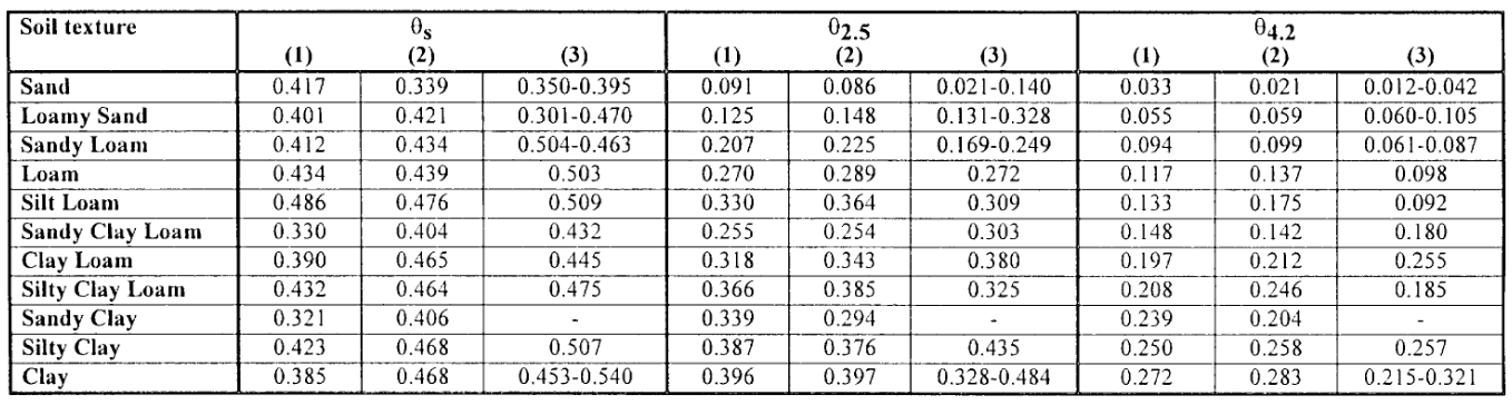
Figure: Moisture content in soil at effective saturation and field capacity/wilting point for different soil types.

Overland flow runoff coefficient CQOF

CQOF is a very important parameter, determining the extent to which excess rainfall runs off as overland flow and the magnitude of infiltration.

CQOF is dimensionless with values between 0 and 1. Physically, in a lumped manner, it reflects the infiltration and also to some extent the recharge conditions. Small values of CQOF are expected for a flat catchment having coarse, sandy soils and a large unsaturated zone, whereas large CQOF-values are expected for catchments having low, permeable soils such as clay or bare rocks. CQOF-values in the range 0.01-0.90 have been experienced.

It should be noted that during periods where the groundwater table is at the ground surface the model excludes the infiltration component, and hence CQOF becomes redundant.

The default value is 0.3.

Time constant for interflow CKIF

CKIF [hours] determines together with U_max the amount of interflow (CKIF)^-1 is the quantity of the surface water content U that is drained to interflow every hour). It is the dominant routing parameter of the interflow because CKIF >> CK₁₂.

Physical interpretation of the interflow is difficult. Since interflow is seldom the dominant streamflow component, CKIF is not, in general, a very important parameter. Usually, CKIF-values are in the range 500-1000 hours.

The default value is 500 hours.

Time constant for routing interflow and overland flow CK₁₂

The time constant for routing interflow and overland flow CK₁₂ [hours] determines the shape of hydrograph peaks. The value of CK₁₂ depends on the size of the catchment and how fast it responds to rainfall. Typical values are in the range 3-48 hours.

The time constant can be inferred from calibration on peak events. If the simulated peak discharges are too low or arriving too late, decreasing CK₁₂ may correct this, and vice versa.

Urban (MIKE+)

From the MIKE+ interface, CK~12 ~are set equal to CK_OF. 

Root zone threshold value for overland flow TOF

TOF is a threshold value for overland flow in the sense that no overland flow is generated if the relative moisture content of the lower zone storage, L/L_max, is less than TOF. The behaviour of the threshold value is illustrated in the generation of overland flow. Similarly, the root zone threshold value for interflow TIF and recharge TG act as threshold values for generation of interflow and recharge, respectively.

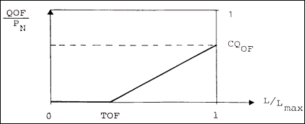
Figure: Generation of overland flow.

Physically, the three threshold values should reflect the degree of spatial variability in the catchment characteristics, so that a small homogeneous catchment is expected to have larger threshold values than a large heterogeneous catchment.

For catchments with alternating dry and wet periods, the threshold values determine the onset of the flow components in the periods where the root zone is being filled up. This can be used in model calibration. It should be noted that the threshold values have no importance in wet periods. The significance of the threshold value varies from catchment to catchment and is usually larger in semi-arid regions.

In areas with alternating dry and wet seasons, TOF can be estimated on the basis of situations where even very heavy rainfall does not give rise to the quick response of the overland flow component. The parameter has an impact only during the first, few weeks of the wet season. Values of TOF in the range 0-0.7 have been experienced.

The default value is 0.

Root zone threshold value for interflow TIF

The root zone threshold value for interflow has the same function for interflow as TOF has for the overland flow. It is usually not a very important parameter, and it can in most cases be given a value equal to zero.

Groundwater parameters

Baseflow time constant CK_BF

The time constant for baseflow, CK_BF [hours], determines the shape of the simulated hydrograph in dry periods. According to the linear reservoir description the discharge in such periods is given by an exponential decay. CK_BF can be estimated from hydrograph recession analysis. CK_BF-values in the range 500-5000 hours have been experienced.

If the recession analysis indicates that the shape of the hydrograph changes to a slower recession after a certain time, an additional (lower) groundwater storage can be added to improve the description of the baseflow.

The default value is 2000 hours.

Root zone threshold value for groundwater recharge TG

The root zone threshold value for recharge has the same effect on recharge as TOF has on the overland flow. It is an important parameter for simulating the rise of the groundwater table in the beginning of a wet season.

Recharge to lower groundwater storage CQ_LOW

River (MIKE 11 / MIKE HYDRO)

In some cases the shape of the hydrograph recession changes to a slower recession after a certain period. To simulate this, a lower groundwater storage may be included. The parameter CQ_LOW determines the proportion of the recharge that percolates to the lower groundwater storage. CQ_LOW together with CK_low can be estimated from hydrograph recession analysis.

The default value is 1000 hours.

Time constant for routing lower baseflow CK_low

River (MIKE 11 / MIKE HYDRO)

The baseflow from the lower groundwater storage is modelled using a linear reservoir with time constant CK_low [hours]. The time constant can be estimated from hydrograph recession analysis. Usually, CK_low is larger than CK_BF.

The default value is 10,000 hours.

Ratio of groundwater catchment to topographical catchment area C_area

Drainage to or from neighbouring catchments can be modelled by specifying a value of C_area different from 1. C_area specifies the amount of recharge G that is being drained. If C_area < 1, part of the recharge, (1-C_area)G, is drained to another catchment, whereas for C_area > 1, the amount (C_area-1)G is added to the catchment recharge.

The default value is 1.

Maximum groundwater depth causing baseflow GWL_BF0

The maximum depth to the groundwater table for which baseflow occurs, GWL_BF0 [m], represents the outflow level of the groundwater reservoir given as the distance between the average ground level of the catchment and the minimum level of the river to which it drains. In low, flat areas the annual variation of this distance may be of importance and the facility to allow GWL_BF0 to vary seasonally is provided in NAM.

GWL_BF0 and the specific yield S_Y can be calibrated by comparing the simulated groundwater level with observations.

The default value is 10 metres.

Specific yield S_Y

Values of the specific yield for the groundwater storage may often be assessed from hydrological data e.g. pump tests. Alternatively, S_Y-values can be estimated from the literature for different soil types. Small values are found for clay (0.01-0.1) and high values for sand (0.1-0.3).

The default value is 0.1.

Groundwater depth for unit capillary flux GWL_FL1

GWL_FL1 [m] is the depth to the groundwater table which yields an upward capillary flux of 1 mm/day when the moisture content of the upper soil layers is at wilting point, i.e. L = 0. This parameter will depend on the soil type, and values for 20 soil types according to Rijtema (1969) ¹³ are listed in the depth to the groundwater table corresponding to a capillary flux of 1 mm/day for 20 soil.

The default value is 0 metre.

Table: Depth to the groundwater table corresponding to a capillary flux of 1 mm/day for 20 soil types.

Soil Type	GWL~FL1 ~[m]
1.  Coarse sand	0.5
2.  Medium coarse sand	0.6
3.  Medium fine sand	0.9
4.  Fine sand	1.5
5.  Humus loamy medium coarse sand	1.2
6.  Light loamy medium coarse sand	0.7
7.  Loamy medium coarse sand	0.5
8.  Loamy fine sand	1.7
9.  Sandy loam	0.7
10.  Loess loam	1.5
11.  Fine sandy loam	2.5
12.  Silty loam	2.8
13.  Loam	1.9
14.  Sandy clay loam	2.2
15.  Silty Clay Loam	1.8
16.  Clayey Loam	1.0
17.  Light clay	2.9
18.  Basin clay	0.4
19.  Silty clay	1.4
20.  Peat	0.6

Minimum groundwater depth for diverting recharge to surface GWL_min

Urban (MIKE+)

Minimal depth of groundwater below surface, at which the groundwater recharge is diverted to the surface/overland flow.

This parameter is not available from the MIKE 11 user interface, therefore the default value of 0.00 metre will apply.

Snow module parameters

Degree-day coefficient C_snow

The snow melts at a rate defined by the degree-day coefficient C_snow [mm /°C/day]. A seasonal variation of C_snow can be defined in order to account for the seasonal variations of the incoming short wave radiation and the albedo of the snow surface. Typical values of C_snow are in the range 2-4 mm/°C/day.

The default value is 3 mm/°C/day.

Base temperature (snow/rain) T₀

River (MIKE 11 / MIKE HYDRO)

The precipitation is assumed to fall as snow if the temperature is below the base temperature T₀ [°C]. For temperatures above T₀ the snow in the snow storage is melting. The base temperature is usually close to zero degrees Celsius.

Radiation coefficient C_rad

River (MIKE 11 / MIKE HYDRO)

The radiation coefficient C_rad [m²/W/mm/day] determines the rate of snow melting caused by the absorbed short wave radiation.

Rainfall degree-day coefficient C_rain

River (MIKE 11 / MIKE HYDRO)

The rainfall degree-day coefficient C_rain [mm/mm/°C/day] determines the rate of snow melting caused by condensation of humid air on the snow surface and the advective heat transferred to the snow pack by precipitation.

Irrigation module parameters

Infiltration factor K0_inf

River (MIKE 11 / MIKE HYDRO)

K0_inf [mm/day] is the infiltration factor which, together with the moisture content in the upper and root zone storages, determines the amount of water infiltrating from the surface to the root zone and groundwater storage.

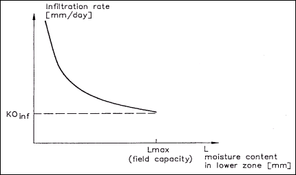
Figure: Infiltration rate as a function of the moisture content in the root zone.

In the infiltration rate as a function of the moisture content in the root zone the infiltration rate is shown as a function of the moisture content in the root zone. K0_inf is strongly dependent on the soil type and is large for sandy soils and small for clayey soils.

When irrigation water is supplied, the root zone will often be close to saturation. Under such conditions the infiltration rate K0_inf may converge to the saturated hydraulic conductivity of the soil (K_s). As a guideline K_s-values for different soil types, as estimated by various authors, are presented in the values of saturated hydraulic conductivity Ks for eleven textural classes from six sources.

When the root zone is only partly saturated, the flow dynamics become very complicated and are not properly described in a lumped model like NAM. Furthermore, the soil preparation may have a significant influence on the soil hydraulic conductivity.

Crop coefficients and irrigation losses

The crop coefficients account for the fact that potential evapotranspiration is dependent of the crop type and the stage of growth. This is achieved by multiplying the input time series of potential evapotranspiration with the crop coefficient. For dry uncropped soils, the crop coefficient will tend to zero while well cropped fields reaching full growth potential could have crop coefficients greater than 1. Further information about how to estimate the crop coefficients is given in ¹¹. Monthly values of crop coefficients can be specified.

The monthly magnitude and distribution of losses to evaporation, seepage, and overland flow should correspond to the design values of the irrigation scheme unless observations have shown a different distribution.

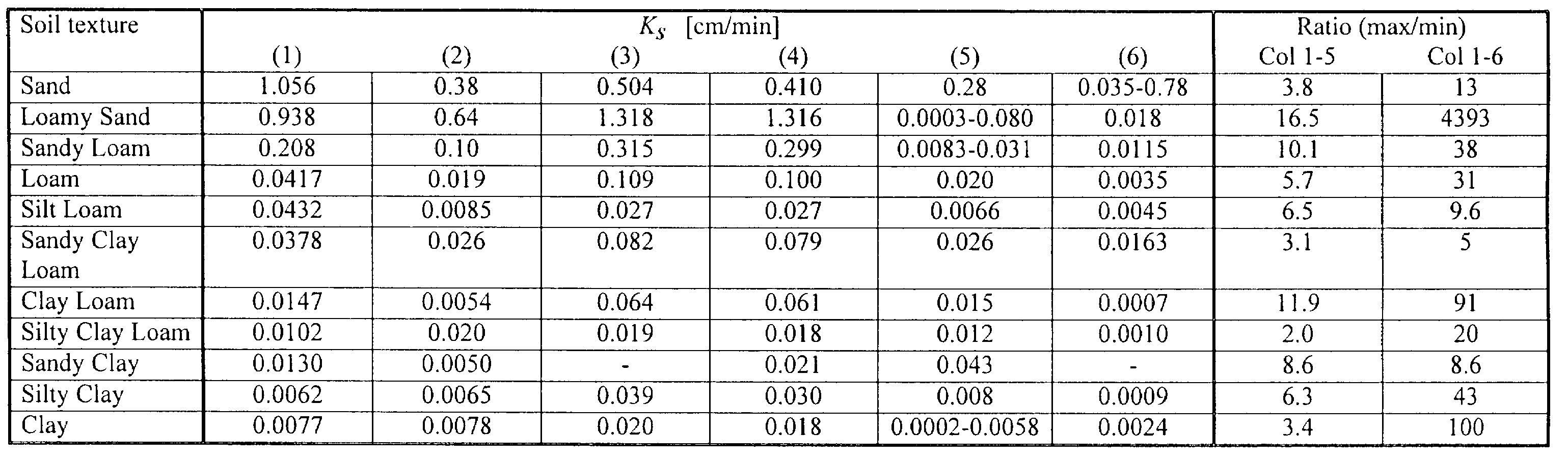
Figure: Values of saturated hydraulic conductivity Ks for eleven textural classes from six sources: (1) Li et al. (1976)⁶; (2) Brakensiek (1979)²; (3) Brakensiek et al. (1981)³; (4) McCuen et al. (1981)⁸; (5) Cosby et al. (1984)⁴; (6) Rijtema (1969)¹³.

Initial conditions

River (MIKE 11 / MIKE HYDRO)Urban (MIKE+)

From the MIKE 11 interface, the initial conditions required by the NAM model consist of the initial water contents in the surface and root zone storages, together with initial values of overland flow, interflow, and baseflow. If a lower groundwater reservoir is specified, the initial baseflow from both the upper and the lower reservoir should be specified.

However from the MIKE+ interface, the water depth of surface and lower zone storage, values of interflow and overland flow and the groundwater depth at the start of the simulation are part of the initial conditions. The groundwater depth, GWL, is related to the NAM parameter GWL_BF0, defining the groundwater depth which generates a groundwater recharge of zero, e.g. a value of 9.5 m for GWL is suitable if the parameter GWL_BF0 is set to 10.0 m, a standard value in NAM model. When changing the values of Umax and Lmax, correspondingly the initiation values Uinit and Linit have to be changed.

If the snow module is included, the initial value of the snow storage should be specified.

If a simulation commences at the end of a dry period, it is often sufficient to set all initial values to zero, except the water content in the root zone and the baseflow. The water content in the root zone should be about 10-30% of the capacity and the baseflow should be given a value close to the observed discharge.

Improved estimates of the initial conditions may be obtained from a previous simulation, covering several years, by noting the appropriate water contents of the root zone and baseflow at the same time of the year as the new simulation will start.

In general it is recommended to disregard the first 3-6 months of the NAM simulation in order to eliminate the influence of erroneous initial conditions.

Model calibration

In the NAM model the parameters and variables represent average values for the entire catchment. While in some cases a range of likely parameter values can be estimated, it is not possible, in general, to determine the values of the NAM parameters on the basis of the physiographic, climatic and soil physical characteristics of the catchment, since most of the parameters are of an empirical and conceptual nature. Thus, the final parameter estimation must be performed by calibration against time series of hydrological observations.

Calibration objectives and evaluation measures

The following objectives are usually considered in the model calibration:

1. A good agreement between the average simulated and observed catchment runoff (i.e. a good water balance)

2. A good overall agreement of the shape of the hydrograph

3. A good agreement of the peak flows with respect to timing, rate and volume

4. A good agreement for low flows

In this respect it is important to note that, in general, trade-offs exist between the different objectives. For instance, one may find a set of parameters that provide a very good simulation of peak flows but a poor simulation of low flows, and vice versa.

In the calibration process, the different calibration objectives 1-4 should be taken into account. If the objectives are of equal importance, one should seek to balance all the objectives, whereas in the case of priority to a certain objective this objective should be favoured.

For a general evaluation of the calibrated model, the simulated runoff is compared with discharge measurements. For individual calibration of the groundwater parameters, the simulated average groundwater level can be compared with groundwater level measurements in the catchments.

Both graphical and numerical performance measures should be applied in the calibration process. The graphical evaluation includes comparison of the simulated and observed hydrograph, and comparison of the simulated and observed accumulated runoff. The numerical performance measures include the overall water balance error (i.e. the difference between the average simulated and observed runoff), and a measure of the overall shape of the hydrograph based on the coefficient of determination or Nash-Sutcliffe coefficient ⁹.

\[ R^2 = 1 - \frac{\sum_{i=1}^{N} [Q_{obs,i} - Q_{sim,i}]^2}{\sum_{i=1}^{N} [Q_{obs,i} - \overline{Q}_{obs}]^2} \]

Equation: Nash-Sutcliffe efficiency coefficient evaluating model fit to observations.

Table: Variables for Nash-Sutcliffe efficiency calculation.

Qsim,i	Simulated discharge at time
Qobs,i	Corresponding observed discharge
\(\overline{Q}_{obs}\)	Average observed discharge
R2 = 1	Corresponds to a perfect match

Where:

An exact agreement between simulations and observations must, however, not be expected. The goodness-of-fit of the calibrated model is affected by different error sources, including

1. Errors in meteorological input data

2. Errors in recorded observations

3. Errors and simplifications inherent in the model structure

4. Errors due to the use of non-optimal parameter values

In model calibration only error source (4) should be minimised. In this respect it is important to distinguish between the different error sources since calibration of model parameters may compensate for errors in data and model structure. For catchments with a low quantity or quality of data, less accurate calibration results may have to be accepted.

Satisfactory calibrations over a full range of flows usually require continuous observations of runoff for a period of 3-5 years. Runoff series of a shorter duration, however, will also be useful for calibration, although they do not ensure an efficient calibration of the model. For a proper evaluation of the reliability and hydrological soundness of the calibrated model it is recommended to validate the model on data not used for model calibration (split-sample test). Some general aspects related to calibration and validation of hydrological models are described in Refsgaard a

Manual calibration

The process of model calibration is normally done either manually or by using computer-based automatic procedures. In this section a manual calibration strategy for the NAM model is outlined. Application of an automatic optimisation routine for calibration of the basic NAM model is described in the subsequent section.

In manual calibration, a trial-and-error parameter adjustment is made until satisfactory results are obtained. It is recommended, especially for the less experienced users, to change only one parameter between each trial, so that the effect of the change can be easily discerned. The manual calibration strategy outlined below is based on the different rainfall-runoff process descriptions for calibration of the relevant model parameters, i.e. the parameters that mostly affect the considered process description (see also Section 7.2.8 Model parameters (p. 187)).

A calibration usually commences by adjusting the water balance in the system. The total evapotranspiration over a certain period should correspond to the accumulated net precipitation minus runoff. The evapotranspiration will increase when increasing the maximum water contents in the surface storage U_max and the root zone storage L_max, and vice versa.

The peak runoff events are caused by large quantities of overland flow. The peak volume can be adjusted by changing the overland flow runoff coefficient (CQOF), whereas the shape of the peak depends on the time constant used in the runoff routing (CK₁₂).

The amount of base flow is affected by the other runoff components; a decrease in overland flow or interflow will result in a higher baseflow, and vice versa. The shape of the baseflow recession is a function of the baseflow time constant (CKBF). If the baseflow recession changes to a slower recession after a certain time, a lower groundwater reservoir should be added, including calibration of CQ_low and CK_low.

Initially, the root zone threshold values TOF, TIF and TG can be set to zero. After a first round of calibration of the parameters U_max, L_max, CQOF, CK₁₂ and CKBF, the threshold parameters can be adjusted for further refinement of the simulation results.

For individual calibration of the groundwater parameters GWL_BF0 and S_Y, the simulated groundwater level is compared to observed groundwater levels. Inclusion of the shallow groundwater reservoir description is important in lowland areas, as found e.g. in swamps or river delta areas, where the groundwater table may reach the ground surface during the wet season.

The snow module parameters are calibrated against periods with snowmelt runoff.

Automatic calibration routine

For calibration of the basic NAM model, including the 9 model parameters listed in , an automatic optimization routine is available. The automatic calibration routine is based on a multi-objective optimization strategy in which the four different calibration objectives given above can be optimised simultaneously.

Multi-objective calibration measures

In automatic calibration, the calibration objectives have to be formulated as numerical goodness-of fit measures that are optimised automatically. For the four calibration objectives defined above the following numerical performance measures are used:

1. Agreement between the average simulated and observed catchment runoff: overall volume error.

2. Overall agreement of the shape of the hydrograph: overall root mean square error (RMSE).

3. Agreement of peak flows: average RMSE of peak flow events.

4. Agreement of low flows: average RMSE of low flow events. Overall volume error.

\[ \text{F}_{1}\left(\theta \right) = \left|\frac{1}{N}\sum_{i = 1}^{N}\left(Q_{obs, i} -Q_{sim, i}\left(\theta \right)\right)\right| \]

Equation: Volume error objective function measuring average difference between observed and simulated discharge.

where

Q_obs,i    is the observed discharge at time i

Q_sim,i    is the simulated discharge at time i

q   is the set of model parameters to be calibrated

N    is the number of time steps in the calibration period Overall RMSE.

\[ F_2(\theta) = \left[ \frac{1}{N} \sum_{i=1}^{N} [Q_{obs,i} - Q_{sim,i}(\theta)]^2 \right]^{1/2} \]

Equation: Root mean square error between observed and simulated discharge for calibration evaluation.

The coefficient of determination in Eq. the nash-Sutcliffe efficiency coefficient evaluating model fit to observations is a transformed and normalised measure of the overall RMSE (normalised with respect to the variance of the observed hydrograph). Thus, minimisation of the root mean square error between observed and simulated discharge for calibration corresponds to maximising R². Average RMSE of peak flow events.

\[ F_3(\theta) = \frac{1}{M_p}\sum_{j=1}^{M_p}\left[\frac{1}{n_j}\sum_{i=1}^{n_j}\left[Q_{obs,i}-Q_{sim,i}(\theta)\right]^2\right]^{1/2} \]

Equation: Average root-mean-square error of peak flow events for model calibration and evaluation.

where M_p is the number of peak flow events in the calibration period, and n_j is the number of time steps in event no. j. Peak flow events are defined as periods where the observed discharge is above a given (user-specified) threshold level. Average RMSE of low flow events.

\[ F_3(\theta) = \frac{1}{M_j}\sum_{j=1}^{M_j}\left[\frac{1}{n_j}\sum_{i=1}^{n_j}[Q_{obs,i}-Q_{sim,i}(\theta)]^2\right]^{1/2} \]

Equation: Objective function measuring average root mean square error across peak flow events for model calibration.

where M_l is the number of low flow events in the calibration period. Low flow events are defined as periods where the observed discharge is below a given (user-specified) threshold level.

Optimization algorithm

The multi-objective optimization problem can be formulated as follows

\[ \operatorname*{min}\{\mathrm{F}_{1}(\theta),~\mathrm{F}_{2}(\theta),~\mathrm{F}_{3}(\theta),~\mathrm{F}_{4}(\theta)\} \quad \text{and} \quad \theta~~~\Theta \]

Equation: Multi-objective optimization problem minimizing competing performance objectives.

The optimization problem is said to be constrained in the sense that q is restricted to the feasible parameter space Q. The parameter space is defined as a hypercube by specifying lower and upper limits on each parameter. These limits should be chosen according to physical and mathematical constraints in the model and from modelling experiences.

The solution of the multi-objective optimization problem minimizing competing performance objectives will not, in general, be a single unique set of parameters but will consist of the so-called Pareto set of solutions (non-dominated solutions), according to various trade-offs between the different objectives. The concept of Pareto optimality implies that the entire parameter space Q can be divided into “good” (Pareto optimal) and “bad” solutions, and none of the “good” solutions can be said to be “better” than any of the other “good” solutions. A member of the Pareto set will be better than any other member with respect to some of the objectives, but because of the trade-off between the different objectives it will not be better with respect to other objectives.

In practical applications, the entire Pareto set may be too expensive to calculate, and one is only interested in part of the Pareto optimal solutions. To estimate only a single point of the Pareto front a single-objective optimization problem is defined that aggregates the different objective functions F₁(q) – F₄(q). The applied aggregate measure is the Euclidian distance

\[ F_{agg}(\theta) = \left[ (F_1(\theta) + A_1)^2 + (F_2(\theta) + A_2)^2 + (F_3(\theta) + A_3)^2 + (F_4(\theta) + A_4)^2 \right]^{1/2} \]

Equation: Aggregated multi-objective function for parameter optimization using Euclidean distance.

where A_i are transformation constants. A balanced aggregated measure is defined by assigning transformation constants in the aggregated multi-objective function for parameter optimization using Euclidean such that the different objectives have equal weight in the optimization. The transformation constants are automatically calculated based on the initially generated population of parameter sets in the optimization loop (⁷).

The optimal parameter set is found by minimising the aggregated multi-objective function for parameter optimization using Euclidean with respect to q. Optimization is performed automatically using the shuffled complex evolution (SCE) algorithm (⁵). The SCE method is a global search method in the sense that it is especially designed for locating the global optimum of the objective function and not being trapped in local optima. A detailed description of the algorithm is given in ⁵. Implementation and testing of the algorithm for automatic calibration of the NAM model is described in ⁷.

User specifications

Specifications for the NAM auto-calibration module include:

• Calibration parameters
• Range of calibration parameters
• Objective functions
• Stopping criterion Calibration parameters. The automatic calibration routine includes the 9 model parameters shown in . The user specifies the subset of these parameters that should be calibrated automatically. Range of calibration parameters. For the subset of NAM parameters to be calibrated automatically the user specifies the hypercube search space, i.e. lower and upper bounds on each parameter. The range of the different parameters should reflect the prior knowledge of experienced values for the type of catchment being considered. Default limits based on physical and mathematical model constraints and experienced values for a range of different catchments are provided in the calibration parameters and default hypercube search space.

Table: Calibration parameters and default hypercube search space.

Parameter	Unit	Lower bound	Upper bound
Umax	[mm]	5	35
Lmax	[mm]	50	400
CQOF	[-]	0	1
CKIF	[hours]	200	2000
CK12	[hours]	3	72
TOF	[-]	0	0.9
TIF	[-]	0	0.9
TG	[-]	0	0.9
CKBF	[hours]	500	5000

Objective functions. The user can specify any combination of the 4 objective functions: (1) overall water balance error, (2) overall RMSE, (3) peak flow RMSE, and (4) low flow RMSE. For the peak and low flow RMSE the user should specify the threshold levels for defining peak and low flow events, respectively.

The choice of objective functions should reflect the objective of the model simulation. For general hydrological studies, the overall water balance error and overall RMSE is normally applied. If focus of the study is on high or low flows, the peak or low flow RMSE should be included. It is not advised to use only the water balance error for optimisation, since this may provide an unrealistic model calibration. Stopping criterion. The stopping criterion for the optimisation algorithm is the maximum number of model evaluations. The appropriate number of model evaluations depends primarily on the number of calibration parameters and the complexity of the model (interaction between model parameters). A large number of model evaluations are, in general, needed for a complex model with many parameters. This requirement should be balanced against the computing time. For a model calibration that includes all 9 parameters, a maximum number of model evaluations in the range 1000-2000 normally ensures an efficient calibration.

Besides the user-defined stopping criterion, the optimisation algorithm includes a parameter convergence criterion. In this case the optimisation algorithm stops if the entire population of parameter sets in an optimisation loop have converged into the same parameter values.

---

1. Abbott, M.B. and Refsgaard, J.C. (eds): Distributed Hydrological Modelling, Kluwer Academic Press, The Netherlands, 321, 1996. ↩↩

2. Brakensiek, D.L.: Comments on 'Empirical Equations for some soil Hydraulic Properties' by Roger B. Clapp and George M. Hornberger, Water Resources Research, 15 (4), 989-990, 1979. ↩

3. Brakensiek, D.L., Engleman, R.L. and Rawls, W.J.: Variation within texture classes of soil water parameters, Trans. ASAE, 24, 335-339, 1981. ↩

4. Cosby, B.J., Hornberger, G.M., Clapp, R.B. and Ginn, T.R.: A statistical exploration of the relationships of soil moisture characteristics to the physical properties of soils, Water Resources Research, 20 (6), 682-690, 1984. ↩

5. Duan, Q., Sorooshian, S., Gupta, V., 1992, Effective and efficient global optimization for conceptual rainfall-runoff models, Water Resour. Res., 28(4), 1015-1031. ↩↩

6. Li, R.-M., Stevens, M.A. and Simons, D.B.: Solutions to Green-Ampt infiltration equations, J. Irrig. and Drain. Div., Amer. Soc. Civil. Eng., 102 (IR2), 239-248, 1976. ↩

7. Madsen, H. ,1999, Automatic calibration of a conceptual rainfallrunoff model using multiple objectives, Journal of Hydrology, Submitted. ↩↩

8. McCuen, R.H., Rawls, W.J. and Brakensiek, D.L.: Statistical analysis of the Brooks-Corey and Green-Ampt parameters across soil textures, Water Resources Research, 17, 1005-1013, 1981. ↩

9. Nash, I.E. and Sutcliffe, I.V.: River flow forecasting through conceptual models, Part I, Journal of Hydrology, 10, 282-290, 1970. ↩

10. Nielsen, S.A. and E. Hansen: Numerical simulation of the rainfall runoff process on a daily basis. Nordic Hydrology, 4, 171-190, 1973. ↩↩

11. Rawls, W.J., Brakensiek, D.L. and Saxton, K.E.: Estimation of soil water properties, Transactions of the ASAE, 25, 1316-1320, 1982. ↩

12. Refsgaard, J.C. and J. Knudsen: Operational validation and intercomparison of different types of hydrological models. Water Resources Research, 32(7), 2189-2202, 1997. ↩↩

13. Rijtema, P.E.: Soil moisture forecasting, Nota 513, Instituut voor Cultuurtechniek en Waterhuishouding, Wageningen, The Netherlands, 1969. ↩↩↩

14. U.S. Army Corps of Engineers: Snow hydrology: Summary report on snow investigations, 1956. ↩