2D Mapping, Flood Maps

River (MIKE 11 / MIKE HYDRO)

Outlined below is the interpolation routine used to generate the various two dimensional maps. These maps can currently only be setup when running a MIKE 11 setup

The mapping of water levels, water depths, velocities and advection dispersion components from the one-dimensional results to two-dimensional maps are done through a number of steps:

• Interpolation of horizontal 2D cross section end point coordinates at all digitised points and all interpolated water level points.
• Mapping between the horizontal 2D (x,y) coordinate an the river coordinate system (chainage and transversal distance from centre of river).
• Linear interpolation of results in the river coordinate system can then be mapped to the 2D coordinate system.

All cells in the 2D grid can spatially interpolate a bed level, water level etc. by using the interpolation and mapping routines.

Interpolation of Cross Section Coordinates

The network consists of digitised points and cross sections, and the two are related by their chainage value. A typical network can be seen in the typical reach with digitised points and cross sections. The circles illustrate the digitised points. The cross sections are shown as the full drawn lines.

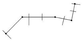
Figure: Typical reach with digitised points and cross sections.

The first step is to obtain a 2D envelope of the river system that follows the digitised points, as in the river 2D envelope

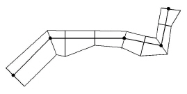
Figure: River 2D envelope.

This is obtained by considering the river as a straight line as in the reach from 1D river coordinates point of view. Dashed lines are interpolated, which is called the river coordinate system. In this river coordinate system, the left/right river width can be interpolated at the digitised points and the interpolated water level points by linear interpolation. The interpolated cross section positions are indicated by dashed lines in the plot.

Figure: Reach from 1D river coordinates point of view. Dashed lines are interpolated river widths at either digitised points or interpolated water level points.

The interpolated widths are used at the digitised points and the interpolated water level points to obtain the 2D horizontal (x,y) coordinates of the river sides, and straight lines between the river side coordinates down the river are used to form the 2D envelope.

Mapping between 2D and 1D Coordinate Systems

The reach is split into a number of segments, bounded by either a digitised point or an interpolated water level point. Each segment has cross section end point coordinates at each end. An actual cross section need not exist at the end of the segments, but further up/down the river. Such a segment is termed a mapping box. the mapping from (x,y) to river system coordinates shows a mapping box in grey and bounded by the dashed lines. In this case cross sections are defined further up/down of the mapping box, indicated by full drawn lines. For each of these mapping boxes a set of local (u,v) coordinate systems are introduced on each side of the river centre line (lowest point line), the mapping from (x,y) to river system coordinates shows one. The (x,y) point in the figure marked with a circle is mapped to the local (u,v) coordinates (0,5;0,5). From this local coordinates it is possible to calculate the river coordinates, chainage and width.

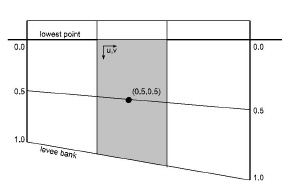
Figure: Mapping from (x,y) to river system coordinates.

For a given (x,y) coordinate, a value is calculated by first mapping the (x,y) coordinate to local (u,v) coordinate system, calculate the river coordinates, and then linearly interpolate the value in the river coordinate system.

When left and/or right bank markers are set, the local mapping needs to take place between each marker line, as in the mapping from (x,y) to river system coordinates when bank markers are specified, hence up to 4 local different (u,v) mappings can take place within a mapping box. Note especially that the relative local river v coordinate differs in each end of the mapping box.

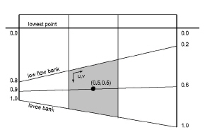
Figure: Mapping from (x,y) to river system coordinates when bank markers are specified.

Linear Interpolation of Results

The interpolation of results at a given grid cell in the 2D map grid depends on the type of result:

• Water levels and concentrations are interpolated between nearest h-points based on the chainage coordinate of the grid cell. Values are only shown if the water level is above the local bed level at the grid cell.
• Water depth is determined as the water level minus the bed level, and will only be shown if the value is positive.
• Velocity is interpolated between the nearest h-points, and is only shown if the water level is above the local bed level at the grid cell.

In all cases results are only provided if the cross sections are open cross sections. Closed cross sections are assumed not to contribute to the map results.

Calculating the Local Velocity Profile in a Grid Point

The velocity distribution in a cross section is assumed to be uniform over the depth and vary as the conveyance in the transversal direction.

The total conveyance K is in this context defined as

\[ K(t) = \int_{0}^{b_{s}(t)}d\left(x,t\right)^{5/3}M(x)\,dx \]

Equation: Total conveyance of a cross section, expressed as the integral of the conveyance density over the wetted width.

where the integration takes place along the cross section profile that is wet, \(b_{s}\) is the width of the cross section, d is the local water depth along the cross section and M is the Manning resistance number. The water depth varies over the cross section, and Manning’s resistance number can also vary over the cross section, but it need not do so. For the Chezy description, the 5/3 is replaced with 3/2 and M is replaced by the Chezy number C

The velocity for a given point in the cross section is defined by

\[ v(x,t) = \frac{q(t)}{K(t)} \cdot M(x) \cdot d(x,t)^{2/3} \]

Equation: Velocity distribution across the cross section width, from the conveyance density.

where the q is the interpolated discharge at the cross section. For the Chezy formulation the M is again replaced by C and the 2/3 s replaced by 1/2.

Hereby a value for the velocity can be found at every point along the cross section, and the velocity in intermediate grid cell points in a mapping box are found by linear interpolation.

For a cross section that does not have raw data defined, or where the cross section is not fully open, above formulation can not take place or is not valid. Instead the velocity result will be just a simple average over the entire cross section and not vary along the cross section.

\[ v(t) = \frac{q(t)}{A_{fl}(h(t))} \]

Equation: Cross-sectional average velocity.