Structures

In general, the structure description in MIKE 1D combines a wide range of elements including weirs, narrow cross sections, flood plains, etc. The concept is based on the calculation of a discharge through the structure as a function of the upstream and downstream water levels, which is then applied on a q-grid point.

MIKE 1D can include structure calculations using two different modes: discharge mode and head loss mode. Not all structures can use both modes. Discharge mode is applicable for all structures. Head loss mode is applicable for Energy equation structures only. Head loss mode is the most recent addition, introduced by Release 2022. Discharge mode corresponds to using the Eqs. the linearised structure discharge at the new time step, expanded around the and (A.2.39) described in Appendix A.2.4.1. Head loss mode corresponds to using Eq. the full momentum equation including the headloss and friction slope terms described in Appendix A.2.4.2.

Energy equation structures supporting head loss mode are:

• Bridges
• Culverts
• Energy loss structures
• Gates
• Broad crested weirs (not Overflow weirs)

For all other structures, the discharge mode is always applied.

The head loss mode is only applicable under sub-critical conditions. If the structure flow is evaluated as super critical, calculations revert to discharge mode.

Discharge mode

The discharge mode is based on the structures explicitly calculating a discharge through the structure q_s, typically based on the surrounding water levels.

\[ q_{s} = f\left(h_{us}, h_{ds}\right) \]

Equation: Structure discharge as a function of upstream and downstream water levels.

Here h_us is the upstream water level and h_ds is the downstream water level. This discharge replaces the evaluation of the momentum equation on a q-grid point. In the simplest form, the structure discharge directly enters Equation the discretised implicit finite-difference form of the momentum equation at a q-grid in the form:

\[ q^{n + \delta} -q^{n} \]

Equation: Change in discharge across a structure in the momentum balance.

Figure: Mathematical notation showing the difference in structure discharge variables.

To increase accuracy and stability, the structure can also calculate derivatives with respect to upstream and downstream water levels, and then the discharge is evaluated for time n+1 as follows:

\[ q^{n+1} = q_{s}^{n} + \frac{dq_{s}^{n}}{dh_{us}}\left(h_{us}^{n+1} - h_{us}^{n}\right) + \frac{dq_{s}^{n}}{dh_{ds}}\left(h_{ds}^{n+1} - h_{ds}^{n}\right) \]

Equation: Linearised structure discharge at the new time step, expanded around the upstream and downstream water levels.

or on the form of Eq. the discretised implicit finite-difference form of the momentum equation at a q-grid:

\[ -\frac{dq_{s}^{n}}{dh_{us}}h_{us}^{n+1} + q^{n+1} - \frac{dq_{s}^{n}}{dh_{ds}}h_{ds}^{n+1} = q_{s}^{n} - \frac{dq_{s}^{n}}{dh_{us}}h_{us}^{n} - \frac{dq_{s}^{n}}{dh_{ds}}h_{ds}^{n} \]

Equation: Linearised structure discharge equation, rearranged with the new time step unknowns on the left.

Which gives:

\[ \alpha_{j} = -\frac{dq_{s}^{n}}{dh_{us}} \]

Equation: Coefficient of the upstream water level in the linearised structure equation.

\[ \beta_{j} = 1 \]

Equation: Coefficient of the discharge in the linearised structure equation.

\[ \gamma_{j} = -\frac{dq_{s}^{n}}{dh_{ds}} \]

Equation: Coefficient of the downstream water level in the linearised structure equation.

\[ \delta_{j} = q_{s}^{n} - \frac{dq_{s}^{n}}{dh_{us}}h_{us}^{n} - \frac{dq_{s}^{n}}{dh_{ds}}h_{ds}^{n} \]

Equation: Constant term in the linearised structure equation.

Head loss mode

In head loss mode, the effect of structures is applied by including an additional head loss term (HL) inside Saint-Venant momentum equation:

\[ \frac{\partial q}{\partial t} + \frac{\partial \left(\alpha\frac{q^{2}}{A}\right)}{\partial x} + gA\frac{\partial h}{\partial x} - ga\frac{HL}{\Delta x} + gAI_{f} = f \]

Equation: The full momentum equation including the headloss and friction slope terms.

with Dx being the distance between to computational h-points surrounding the structure. The advantage of this approach is that it allows for structures with zero head loss, simply by evaluating the HL term to zero. Furthermore, it includes bed friction f between two h-points in the normal way. This approach is especially relevant for structures that do not interact with the flow until at some water level, (e.g. a bridge overflow). Note that the zero head loss scenario the discharge mode cannot handle.

When the flow through the structure becomes critical \(Q \geq Q_{critical}\), the calculations are switched to the discharge mode.

This head loss term is evaluated in the following way:

1. The typical energy equations are solved to determine the structure flow q_s (for example, see Eq. the energy balance for submerged culvert flow accounting for contraction loss). The energy equation usually relates the water level difference and the structure discharge in the following way:

\[ h_{in, s} -h_{out, s} = c\left(h_{in, s}, h_{out, s}, q_{s}\right)q_{s}^{2} \]

Equation: Energy equation relating water level difference across a structure to discharge squared.

• Here we introduce the concept of an overall head loss coefficient c(h_in,s, h_out,s, q_s). This coefficient is a function of inflow and outflow water levels at the structure h_in,s, h_out,s and the structure discharge q_s. For small water level differences h_in,s - h_out,s , we have \(c\left(h_{in,s},h_{out,s},q_{s}\right) \approx c\left(h_{in,s},h_{out,s}\right)\).

• The actual discharge in the structure from previous Saint-Venant equation solution is q_SV=qⁿ. It is used to evaluate a head loss HL=h’_in,s - h’_out,s by assuming that the head loss coefficient (h_in,s, h_out,s, q_s) is the same as from the calculation in point 1.

\[ HL = h'_{in,s} - h'_{out,s} = c\left(h_{in,s},h_{out,s},q_{s}\right)q_{SV}^{2} = \left(h_{in,s} - h_{out,s}\right)\frac{q_{SV}^{2}}{q_{s}^{2}} \]

Equation: Headloss across a structure, expressed through a coefficient function of the water levels and flow.

• We stress that the Saint-Venant discharges qⁿ or qⁿ⁺¹ are not the same as the structure discharge q_s=q_s(h_usⁿ,h_dsⁿ) coming as a solution to the energy equation. However, if a stationary flow state is reached q_SV and q_s do become the same.

• Note that here the inflow/outflow water levels at the structure h_in,s, h_out,s are not upstream/downstream water levels h_us, h_ds of the corresponding H-grid points. The inflow/outflow water levels at the structure are upstream/downstream water levels modified by the friction loss of the flow. This is needed to not double count the effect of the friction loss also appearing in Eq. the full momentum equation including the headloss and friction slope terms. The h_us and h_ds can be modified in a simplified way as

\[ h_{in,s} = h_{us}^{n} - \min\left[\frac{q_{SV}^{2}}{K_{us}^{2}}, k\right]l_{us} \\[1ex] h_{out,s} = h_{ds}^{n} - \min\left[\frac{q_{SV}^{2}}{K_{ds}^{2}}, k\right]l_{ds} \\[1ex] k = \frac{h_{us} - h_{ds}}{l_{us} + l_{ds}} \]

Equation: Water levels at the inlet and outlet of a structure, limited by the upstream/downstream slope.

• Here: l_us/ds distance from upstream/downstream location to the structure, (m) K_us/ds conveyance at the upstream/downstream cross section, (m³/s) - One of the main assumptions for Eq. the water levels at the inlet and outlet of a structure, limited by the to be valid is that the head loss appearing due to flow from upstream cross section to structure and from structure to downstream cross section is considerably smaller than the head loss happening in the structure.

Time discretization of head loss term

The head loss term is dependent on discharge q_SV and inflow/outflow water levels h_us/ds. At discrete time step n+1 it can be Taylor expanded as

\[ HL^{n+1} \approx HL^{n} + \frac{dHL^{n}}{dq_{SV}}\left(q^{n+1} - q^{n}\right) + \left(h_{ds}^{n+1} - h_{ds}^{n}\right) + \frac{dHL^{n}}{dh_{us}}\left(h_{us}^{n+1} - h_{us}^{n}\right) + \frac{dHL^{n}}{dh_{ds}}\left(h_{ds}^{n+1} - h_{ds}^{n}\right) \]

Equation: First-order Taylor expansion of the headloss HL at the new time step.

The head loss derivative with respect to discharge is interpreted as derivative with respect to q_SV and using Eq. the headloss across a structure, expressed through a coefficient function of the it becomes:

\[ \frac{dHL^{n}}{dq_{SV}} \approx \frac{dHL^{n}}{dq_{SV}} = 2\left(h_{in,s} - h_{out,s}\right)\frac{q_{SV}}{q_{s}^{2}} \]

Equation: Derivative of the headloss with respect to discharge.

In the current Mike1D implementation of head loss mode the dHL/dh_us/ds terms are disregarded and only the dHL/dq_SV term is kept in Eq. (A.2.48).

Linearisation of flow when head approaches zero

When the head across the structure approaches zero, a linearisation is used in order to avoid discontinuities. If the difference between up- and down-stream water levels is below the delH, then the discharge and discharge derivatives are linearly interpolated between zero and their value at a water level difference of delH.

General energy headloss considerations

The description generally used for flow through a structure is given by:

\[ \Delta H = \zeta\frac{V_{s}^{2}}{2g} \]

Equation: Headloss expressed through a loss coefficient and the approach velocity head.

where DH is the energy headloss over the structure, z is a headloss coefficient and V_s is the mean cross sectional velocity at the structure.

For broad crested weir, special weir and culverts the headloss is divided into inflow (contraction) and outflow (expansion) components.

In the case of a sudden expansion the energy loss can be described as the headloss expressed through a loss coefficient and the approach velocity head and as:

\[ \Delta H = f\frac{\left(V_{s} - V_{2}\right)^{2}}{2g} \]

Equation: Headloss expressed through the velocity difference across the structure.

Setting the headloss expressed through a loss coefficient and the approach velocity head equal to the headloss expressed through the velocity difference across the structure gives:

\[ \zeta_{2}\frac{V_{s}^{2}}{2g} = f\frac{\left(V_{s} - V_{2}\right)^{2}}{2g} \]

Equation: Equating the two headloss expressions to solve for the loss coefficient.

which can be reduced to:

\[ \zeta_{2} = f\left(1 - \frac{V_{2}}{V_{s}}\right)^{2} \]

Equation: Loss coefficient expressed through the velocity ratio.

f, is equal to the user defined outflow headloss coefficient (z_out) and the loss coefficient expressed through the velocity ratio becomes equal to:

\[ \zeta_{2} = \zeta_{out}\left(1 - \frac{V_{2}}{V_{s}}\right)^{2} \]

Equation: Loss coefficient, generalised with the outlet loss coefficient.

Equation the loss coefficient, generalised with the outlet loss coefficient can also be written in the form:

\[ \zeta_{2} = \zeta_{out}\left(1 - \frac{Q_{2}A_{s}}{A_{2}Q_{s}}\right)^{2} \]

Equation: Loss coefficient expressed through the discharge and area ratios.

Which in case of a single structure (Q_s = Q₂, see the cross-sectional flow areas at a structure showing entrance and exit velocity) is equal to:

\[ \zeta_{2} = \zeta_{out}\left(1 - \frac{A_{s}}{A_{2}}\right)^{2} \]

Equation: Loss coefficient expressed through the area ratio.

For a parallel structure the loss coefficient expressed through the discharge and area ratios cannot be reduced to the loss coefficient expressed through the area ratio as (\(Q_{s} = Q_{2}\)) consequently equation the loss coefficient, generalised with the outlet loss coefficient can be applied instead.

A similar approach can be used for adjustment of inflow headloss:

\[ \zeta_{1} = \zeta_{in}\left(1 - \frac{V_{1}}{V_{s}}\right) \]

Equation: Inlet loss coefficient, expressed through the velocity ratio.

where, z₁ and z₂ are the adjusted inflow and outflow headloss coefficients calculated using the inflow and outflow loss coefficients (z_in and z_out).

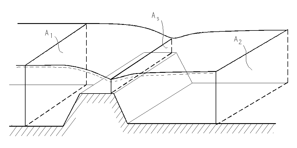
Figure: Cross-sectional diagram showing flow areas at a structure with inflow, outflow, and main flow paths.

River (MIKE 11 / MIKE HYDRO)

A minimum value for z₁ and z₂ can be specified in the HD parameter editor under the Default Values tab as ZetaMin. In the case \(A_{s} \to A_{1}\) the solution can become unstable (no friction) and specification of a minimum value of z_1,2, ensures a stable solution.

Expansion and contraction coefficients

As described in the previous section, flow through a structure is described according to:

\[ \Delta h = \zeta_{t}\frac{Q^{2}}{2gA^{2}} \]

Equation: Total headloss across the structure.

This equation z~ t~ describes the total headloss coefficient, which is composed of entrance (z₁) and exit (z₂) coefficients. For subcritical flow the coefficients are related to the input parameters z_in and z~out ~and the changes in velocity (v) and area (A):

\[ \zeta_{t} = \zeta_{1} + \zeta_{2} = \zeta_{in}\left(1 - \frac{v_{1}}{v_{s}}\right) + \zeta_{out}\left(1 - \frac{A_{s}}{A_{2}}\right)^{2} \]

Equation: Total loss coefficient, combining the inlet and outlet contributions.

For subcritical flow through a structure there is an upstream contraction and a downstream expansion, so equation the total loss coefficient, combining the inlet and outlet contributions works fine. When there is supercritical flow there is an upstream expansion and a downstream contraction. Thus if supercritical flow occurs then the loss coefficients are no longer valid. To accommodate supercritical flow, calculation of the of entrance (z₁) and exit (z₂) coefficients are expanded:

\[ \zeta_{1} = \begin{cases} \zeta_{in}\left(1 - \dfrac{v_{1}}{v_{s}}\right) & \text{for } v_{1} < v_{s} \\[1.5ex] \zeta_{in}\left(1 - \dfrac{A_{1}}{A_{s}}\right)^{2} & \text{for } v_{1} > v_{s} \end{cases} \]

Equation: Inlet headloss coefficient, depending on whether the inlet velocity is below or above the structure's characteristic velocity.

\[ \zeta_{2} = \begin{cases} \zeta_{out}\left(1 - \dfrac{v_{s}}{v_{2}}\right) & \text{for } v_{s} < v_{2} \\[1.5ex] \zeta_{out}\left(1 - \dfrac{A_{s}}{A_{2}}\right)^{2} & \text{for } v_{s} > v_{2} \end{cases} \]

Equation: Outlet headloss coefficient, depending on whether the structure's characteristic velocity is below or above the outlet velocity.

Care must be taken when selecting loss coefficients, particularly in situations where both subcritical and supercritical flow conditions occur. When flow conditions change from subcritical to supercritical (or the Froude number F_R becomes greater than 1), the loss coefficients z_in and z_out (specified in the Headloss Factors box) are modified:

• If F_R > 1 in upstream h-point then z_in = z_in / 2
• If F_R > 1 in downstream h-point then z_out = z_out / 2

Note that this adjustment is not made for bridge structures.

Determination of flow regime

Given the upstream and downstream water levels and the discharge, and assuming that these three values are compatible with each other, the type of flow can be determined as follows.

For zero flow the upstream and downstream water levels are both below the structure invert (crest level) and the flow regime is subcritical, or the flow direction is opposite valve regulation.

For differentiating between critical and drowned flow it is assumed, in the first instance, that the flow at the weir crest is critical.

The critical discharge is determined for broad crested weirs, special weirs and culverts via the tabulated QH-relation while it in case of structures with time dependent geometry is computed by critical flow iteration during the simulation. The pre-processed QH-relation for broad crested weirs are based on the assumption of a single structure, hence when the broad crested weir is a part of a composite structure the QH-relation is no longer valid. In this case the critical discharge is computed by iteration during the simulation. When special weirs and culverts are included in a composite structure it is assumed that the user defined QH-relations for critical flow takes the changed hydraulic conditions into account. When the upstream flow regime is supercritical, the QH-relations are also recalculated.

When a long culvert is a part of a composite structure, there is no critical discharge iteration i.e. the computed QH-relation is used to estimate the critical discharge. This approach is assumed valid as the structure area usually is much smaller than the upstream area i.e. \(A_{s} \ll A_{1}\) hence no need for iteration.

Critical flow occurs (for z₂ > 1) when the energy head at the crest is larger than the downstream energy head, viz.:

\[ h_{s} + \left(1 - \zeta_{2}\right)\frac{Q_{s}^{2}}{2gA_{s}^{2}} \geq h_{2} + \frac{Q_{s}^{2}}{2gA_{2}^{2}} \]

Equation: Energy condition for critical flow over a weir or submerged structure.

Critical flow occurs (for \(\zeta_{2} \leq 1\) and outflow headloss less or equal to 1) when the water level at the crest is larger than the downstream energy head:

\[ h_{s} \geq h_{2} + \frac{Q_{s}^{2}}{2gA_{2}^{2}} \]

Equation: Critical flow condition where upstream energy head exceeds downstream energy head at the structure crest.

If the flow is not critical, a submerged discharge iteration is performed and the submerged discharge is compared with the critical and the smallest is taken.

Discharge over specific structures

How the discharge and the discharge derivatives over specific structures for use in equation (A.2.39) are calculated is not presented in this document for all structures.

Section B.1 QH Relations Calculated for Culverts (p. 317) presents some details for culverts.