Fully dynamic MIKE

Fully dynamic, MIKE+

The momentum term is approximated based on the transformation introduced by Abbott and Ionescu (¹):

\[ \frac{\partial \left(\frac{q^{2}}{A}\right)}{\partial x} = \frac{\partial \left(q \cdot qA^{-1}\right)}{\partial x} = qA^{-1}\frac{\partial q}{\partial x} + Q\frac{\partial \left(qA^{-1}\right)}{\partial x} \]

Equation: Momentum term after the Abbott-Ionescu transformation.

Using the Continuity Equationthe continuity equation in terms of discharge and water level with slot storage to eliminate the q derivative gives:

\[ \frac{\partial \left(\frac{q^{2}}{A}\right)}{\partial x} = qA^{-1}\left(-b_{s}\frac{\partial h}{\partial t} + q_{in}\right) + Q\frac{\partial \left(qA^{-1}\right)}{\partial x} \]

Equation: Momentum term with the discharge derivative eliminated using the continuity equation.

The last term is approximated at time \(n + \delta\), when available, though in first iteration at time n:

\[ Q\frac{\partial \left(qA^{-1}\right)}{\partial x} \approx \left( (1-\delta) q^{n} + \delta q^{n+\delta} \right) \cdot \left( \frac{\left(\frac{q}{A}\right)_{j+1}^{n+\delta} - \left(\frac{q}{A}\right)_{j-1}^{n+\delta}}{\Delta x} \right) \]

Equation: Discretised approximation of the convective acceleration term.

The resistance term in the fully dynamic MIKE+ scheme has several approximations, depending on the resistance formulation. If the resistance formulation is Manning M, in MIKE+ terms called explicit Manning, the term is included in the form:

\[ I_{f} = \frac{\sqrt{I_{h}}}{MAR^{2/3}} \]

Equation: Friction slope term for the explicit Manning resistance formulation.

The user can also specify to use an implicit Manning formulation, in which case the friction term is approximated using the higher order approximation of Verwer, described in Section A.2.1.3.

The 1D engine currently only supports the explicit Manning formulation.

Urban (MIKE+)

In MIKE+, the choice between explicit and implicit flow resistance description is made through the DHIAPP.INI file, see Appendix D.3. The explicit description is selected per default.

Implicit resistance implementation

The resistance term can be approximated using the higher order accurate approximation of Verwer, ⁴. This higher order accurate approximation can greatly improve the stability of the scheme. It is based on a resistance formulation on the form

\[ I_{f} = F = fq\left|q\right| \]

Equation: Friction slope expressed as the momentum forcing term.

where f is a generalised friction factor. The resistance term is approximated at time step n+\(\delta\), i.e. time \(t^{n} + \delta \cdot \Delta t\), using a Taylor expansion around time \(f^{n}\), remembering that the friction factor \(f = f\left(h\right)\) depends on the water level h:

\[ F(t^{n} + \delta \Delta t) = F(t^{n}) + \delta \Delta t\frac{\partial F}{\partial t} = F(t^{n}) + \delta \Delta t\left(\frac{\partial F}{\partial q} \cdot \frac{\partial q}{\partial t} + \frac{\partial F}{\partial h} \cdot \frac{\partial h}{\partial t}\right) \]

Equation: Taylor expansion of the friction term in time.

In terms of values at the time step n, it becomes

\[ F^{n+\delta} \approx F^{n} + \delta\left(\left.\frac{\partial F}{\partial q}\right|^{n} \cdot \Delta q + \left.\frac{\partial F}{\partial h}\right|^{n} \cdot \Delta h\right) \]

Equation: Taylor series expansion approximating friction term evolution through fractional time step.

Expanding this gives

\[ F^{n+\delta} \approx f^{n}\left|q^{n}\right|q^{n} + \delta\left(2f^{n}\left|q^{n}\right| \cdot (q^{n+\delta} - q^{n}) + \left|q^{n}\right|q^{n}\left.\frac{\partial f}{\partial h}\right|^{n} \cdot \Delta h\right) \]

Equation: Taylor expansion of friction force separating explicit and implicit components with resistance derivatives.

The friction factor derivative depends on the resistance formulation. For Manning M and Chezy, the factor is based on the conveyance,

\[ K = K(h) = MAR^{2/3} \quad \text{or} \quad CAR^{1/2} \]

Equation: Conveyance for the Manning M or Chezy C resistance formulation.

where

\[ f = \frac{1}{K^{2}} = M^{-2}A^{-2}R^{-4/3} \quad \text{or} \quad C^{-2}A^{-2}R^{-1} \]

Equation: Friction factor for the Manning M or Chezy C resistance formulation.

This gives the friction factor derivatives:

\[ \frac{\partial f}{\partial h} = -2M^{-3}\frac{\partial M}{\partial h}A^{-2}R^{-4/3} - 2M^{-2}A^{-3}\frac{\partial A}{\partial h}R^{-4/3} - \frac{4}{3}M^{-2}A^{-2}R^{-1}\frac{\partial R}{\partial h} \]

Equation: Derivative of the friction factor with respect to water level, Manning M formulation.

\[ \frac{\partial f}{\partial h} = -2C^{-3}\frac{\partial C}{\partial h}A^{-2}R^{-1} - 2C^{-2}A^{-3}\frac{\partial A}{\partial h}R^{-1} - C^{-2}A^{-2}R^{-2}\frac{\partial R}{\partial h} \]

Equation: Derivative of the friction factor with respect to water level, Chezy C formulation.

which can be simplified to

\[ \frac{\partial f}{\partial h} = f\left(-2M^{-1}\frac{\partial M}{\partial h} - 2A^{-1}\frac{\partial A}{\partial h} - \frac{4}{3}R^{-1}\frac{\partial R}{\partial h}\right) \]

Equation: Simplified derivative of the friction factor, Manning M formulation.

\[ \frac{\partial f}{\partial h} = f\left(-2C^{-1}\frac{\partial C}{\partial h} - 2A^{-1}\frac{\partial A}{\partial h} - R^{-1}\frac{\partial R}{\partial h}\right) \]

Equation: Simplified derivative of the friction factor, Chezy C formulation.

The \(\Delta h\) term is approximated at the h grid point in the flow upstream direction, i.e.

\[ \Delta h = h_{us}^{n+1} - h_{us}^{n-1} \]

Equation: Water level increment used for the time-centred friction term.

where

\[ h_{us} = \begin{cases} h_{j-1} & \text{if } (q_{j} > 0) \\[1ex] h_{j+1} & \text{if } (q_{j} < 0) \end{cases}, \quad h_{ds} = \begin{cases} h_{j+1} & \text{if } (q_{j} > 0) \\[1ex] h_{j-1} & \text{if } (q_{j} < 0) \end{cases} \]

Equation: Upstream and downstream water levels, taken from the upwind grid point.

The coefficient d determines the time weighting of the scheme. For stability reasons the coefficient should be above 0.5.

Node Equations

In nodes a continuity equation covering the surrounding h- and q-grid points is set up. the node with three reaches connected to it gives a close look at the grid points surrounding a node.

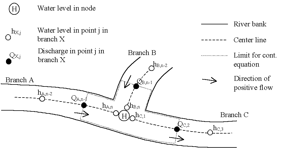
Figure: Grid points surrounding a node in the numerical scheme.

The finite difference approximation of the continuity equation around the node is given by:

\[ \frac{H^{n+1} - H^{n}}{\Delta t}A_{fl} = q_{I}^{n+\frac{1}{2}} - q_{O}^{n+\frac{1}{2}} \Rightarrow \frac{H^{n+1} - H^{n}}{\Delta t}A_{fl} = \frac{1}{2}\left(q_{A,n-1}^{n} + q_{B,n-1}^{n} - q_{C,2}^{n}\right) + \frac{1}{2}\left(q_{A,n-1}^{n+1} + q_{B,n-1}^{n+1} - q_{C,2}^{n+1}\right) \]

Equation: Node continuity equation, time-centred between inflow and outflow contributions.

where

q_ISum of inflows

q_OSum of outflows

Dt Time step

Including Boundaries in the Equations

The following three types of boundary conditions can be applied:

• Water level as a function of time
• Discharge as a function of time
• A tabulated relation between water level and discharge (Q/h boundary)

Each of the boundary types is taken into account by using a different node equation.

Water level as a function of time

In this case the water level in the node at time step n+1 simply becomes the value of the user-specified boundary at time step n+1 (\(H_{boundary}^{n + 1}\)) i.e. in the relevant equation (or row) in the node matrix only the diagonal and the right hand side coefficient are different from zero, and equals respectively 1 and \(H_{boundary}^{n + 1}\).

Discharge as function of time

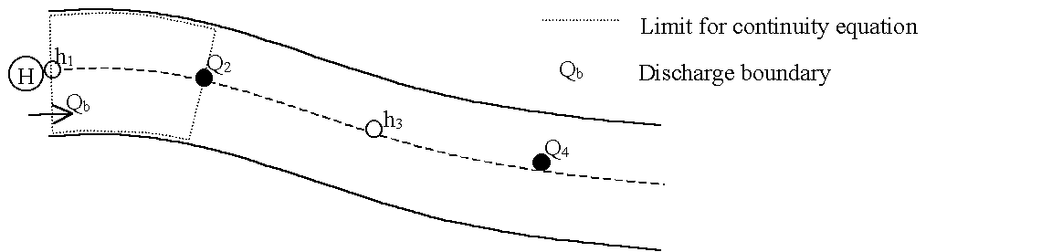
Figure: Reach with discharge boundary.

Figure: Reach cross-section with discharge boundary condition. In this case a local continuity equation covering the area indicated in the reach with discharge boundary is set up. Equation (A.2.30) becomes:

\[ \frac{H^{n+1} - H^{n}}{\Delta t}A_{fl} = \frac{1}{2}\left(q_{b}^{n} - q_{2}^{n}\right) + \frac{1}{2}\left(q_{b}^{n+1} - q_{2}^{n+1}\right) \]

Equation: Node continuity equation, time-centred between the tabulated inflow and outflow.

QH Boundary

In this case the user specifies a tabulated relation between h and Q. A continuity equation is set up at the boundary in the same way as for a discharge boundary. The discharge at the boundary q_b is expressed as a function of the water level in the node using the tabulated relation. This is done as follows:

The index i is found such that \(H_{tab,i} \leq H^{n} < H_{tab,i+1}\), and the ratio a is calculated according to equation the slope for linear interpolation of discharge between tabulated water level values.

\[ a = \frac{q_{\text{tab,i+1}} -q_{\text{tab,i}}}{H_{\text{tab,i+1}} -H_{\text{tab,i}}} \]

Equation: Slope for linear interpolation of discharge between tabulated water level values.

Using linear interpolation between the tabulated values of water levels and discharge equations the breach discharge from linear interpolation between tabulated water level and and (A.2.34) can be achieved:

\[ q_{b}^{n + 1} = q_{\text{tab,i}} + a\left(H^{n + 1} -H_{\text{tab,i}}\right) \]

Equation: Breach discharge from linear interpolation between tabulated water level and discharge values.

\[ q_{b}^{n} = q_{tab,i} + a\left(H^{n} - H_{tab,i}\right) \]

Equation: Structure discharge interpolated from the QH table.

Equations the breach discharge from linear interpolation between tabulated water level and and (A.2.34) are substituted into equation the node continuity equation, time-centred between the tabulated inflow and outflow and equation (A.2.35) is achieved:

\[ \frac{H^{n+1} - H^{n}}{\Delta t}A_{fl} = \frac{1}{2}\left(q_{tab,i} + a\left(H^{n} - H_{tab,i}\right) - q_{2}^{n}\right) + \frac{1}{2}\left(q_{tab,i} + a\left(H^{n+1} - H_{tab,i}\right) - q_{2}^{n+1}\right) \]

Equation: Node continuity equation with the tabulated discharge substituted in.

Structures

In general, the structure description in MIKE 1D combines a wide range of elements including weirs, narrow cross sections, flood plains, etc. The concept is based on the calculation of a discharge through the structure as a function of the upstream and downstream water levels, which is then applied on a q-grid point.

MIKE 1D can include structure calculations using two different modes: discharge mode and head loss mode. Not all structures can use both modes. Discharge mode is applicable for all structures. Head loss mode is applicable for Energy equation structures only. Head loss mode is the most recent addition, introduced by Release 2022. Discharge mode corresponds to using the Eqs. the linearised structure discharge at the new time step, expanded around the and (A.2.39) described in Appendix A.2.4.1. Head loss mode corresponds to using Eq. the full momentum equation including the headloss and friction slope terms described in Appendix A.2.4.2.

Energy equation structures supporting head loss mode are:

• Bridges
• Culverts
• Energy loss structures
• Gates
• Broad crested weirs (not Overflow weirs)

For all other structures, the discharge mode is always applied.

The head loss mode is only applicable under sub-critical conditions. If the structure flow is evaluated as super critical, calculations revert to discharge mode.

Discharge mode

The discharge mode is based on the structures explicitly calculating a discharge through the structure q_s, typically based on the surrounding water levels.

\[ q_{s} = f\left(h_{us}, h_{ds}\right) \]

Equation: Discharge through a structure as a function of upstream and downstream water levels.

Here h_us is the upstream water level and h_ds is the downstream water level. This discharge replaces the evaluation of the momentum equation on a q-grid point. In the simplest form, the structure discharge directly enters Equation the discretised implicit finite-difference form of the momentum equation at a q-grid in the form:

\[ q^{n + \delta} -q^{n} \]

Equation: Discharge increment introduced by a structure into the momentum equation.

The superscript for the structure discharge, \(\tilde{n}\), indicates that the structure flow is evaluated at time n. However, when more than one iteration per time step is applied, this can optionally be changed to evaluate using the intermediate iteration solution at time \(n + delta\), or \(n + 1\).

To increase accuracy and stability, the structure can also calculate derivatives with respect to upstream and downstream water levels, and then the discharge is evaluated for time n+1 as follows:

\[ q^{n+1} = q_{s}^{n} + \frac{dq_{s}^{n}}{dh_{us}}\left(h_{us}^{n+1} - h_{us}^{n}\right) + \frac{dq_{s}^{n}}{dh_{ds}}\left(h_{ds}^{n+1} - h_{ds}^{n}\right) \]

Equation: Linearised structure discharge at the new time step, expanded around the upstream and downstream water levels.

or on the form of Eq. the discretised implicit finite-difference form of the momentum equation at a q-grid:

\[ -\frac{dq_{s}^{n}}{dh_{us}}h_{us}^{n+1} + q^{n+1} - \frac{dq_{s}^{n}}{dh_{ds}}h_{ds}^{n+1} = q_{s}^{n} - \frac{dq_{s}^{n}}{dh_{us}}h_{us}^{n} - \frac{dq_{s}^{n}}{dh_{ds}}h_{ds}^{n} \]

Equation: Linearised structure discharge equation, rearranged with the new time step unknowns on the left.

Which gives:

\[ \alpha_{j} = -\frac{dq_{s}^{n}}{dh_{us}} \]

Equation: Coefficient of the upstream water level in the linearised structure equation.

\[ \beta_{j} = 1 \]

Equation: Coefficient of the discharge in the linearised structure equation.

\[ \gamma_{j} = -\frac{dq_{s}^{n}}{dh_{ds}} \]

Equation: Coefficient of the downstream water level in the linearised structure equation.

\[ \delta_{j} = q_{s}^{n} - \frac{dq_{s}^{n}}{dh_{us}}h_{us}^{n} - \frac{dq_{s}^{n}}{dh_{ds}}h_{ds}^{n} \]

Equation: Constant term in the linearised structure equation.

Head loss mode

In head loss mode, the effect of structures is applied by including an additional head loss term (HL) inside Saint-Venant momentum equation:

\[ \frac{\partial q}{\partial t} + \frac{\partial \left(\alpha\frac{q^{2}}{A}\right)}{\partial x} + gA\frac{\partial h}{\partial x} - ga\frac{HL}{\Delta x} + gAI_{f} = f \]

Equation: The full momentum equation including the headloss and friction slope terms.

with Dx being the distance between to computational h-points surrounding the structure. The advantage of this approach is that it allows for structures with zero head loss, simply by evaluating the HL term to zero. Furthermore, it includes bed friction f between two h-points in the normal way. This approach is especially relevant for structures that do not interact with the flow until at some water level, (e.g. a bridge overflow). Note that the zero head loss scenario the discharge mode cannot handle.

When the flow through the structure becomes critical \(Q \geq Q_{critical}\), the calculations are switched to the discharge mode.

This head loss term is evaluated in the following way:

1. The typical energy equations are solved to determine the structure flow q_s (for example, see Eq. the energy balance for submerged culvert flow accounting for contraction loss). The energy equation usually relates the water level difference and the structure discharge in the following way:

\[ h_{in, s} -h_{out, s} = c\left(h_{in, s}, h_{out, s}, q_{s}\right)q_{s}^{2} \]

Equation: Energy equation relating head loss across a structure to discharge.

• Here we introduce the concept of an overall head loss coefficient c(h_in,s, h_out,s, q_s). This coefficient is a function of inflow and outflow water levels at the structure h_in,s, h_out,s and the structure discharge q_s. For small water level differences h_in,s - h_out,s , we have \(c\left(h_{in,s},h_{out,s},q_{s}\right) \approx c\left(h_{in,s},h_{out,s}\right)\).

• The actual discharge in the structure from previous Saint-Venant equation solution is q_SV=qⁿ. It is used to evaluate a head loss HL=h’_in,s - h’_out,s by assuming that the head loss coefficient (h_in,s, h_out,s, q_s) is the same as from the calculation in point 1.

\[ HL = h'_{in,s} - h'_{out,s} = c\left(h_{in,s},h_{out,s},q_{s}\right)q_{SV}^{2} = \left(h_{in,s} - h_{out,s}\right)\frac{q_{SV}^{2}}{q_{s}^{2}} \]

Equation: Headloss across a structure, expressed through a coefficient function of the water levels and flow.

• We stress that the Saint-Venant discharges qⁿ or qⁿ⁺¹ are not the same as the structure discharge q_s=q_s(h_usⁿ,h_dsⁿ) coming as a solution to the energy equation. However, if a stationary flow state is reached q_SV and q_s do become the same.

• Note that here the inflow/outflow water levels at the structure h_in,s, h_out,s are not upstream/downstream water levels h_us, h_ds of the corresponding H-grid points. The inflow/outflow water levels at the structure are upstream/downstream water levels modified by the friction loss of the flow. This is needed to not double count the effect of the friction loss also appearing in Eq. the full momentum equation including the headloss and friction slope terms. The h_us and h_ds can be modified in a simplified way as

\[ h_{in,s} = h_{us}^{n} - \min\left[\frac{q_{SV}^{2}}{K_{us}^{2}}, k\right]l_{us} \\[1ex] h_{out,s} = h_{ds}^{n} - \min\left[\frac{q_{SV}^{2}}{K_{ds}^{2}}, k\right]l_{ds} \\[1ex] k = \frac{h_{us} - h_{ds}}{l_{us} + l_{ds}} \]

Equation: Water levels at the inlet and outlet of a structure, limited by the upstream/downstream slope.

• Here: l_us/ds distance from upstream/downstream location to the structure, (m) K_us/ds conveyance at the upstream/downstream cross section, (m³/s) - One of the main assumptions for Eq. the water levels at the inlet and outlet of a structure, limited by the to be valid is that the head loss appearing due to flow from upstream cross section to structure and from structure to downstream cross section is considerably smaller than the head loss happening in the structure.

Time discretization of head loss term

The head loss term is dependent on discharge q_SV and inflow/outflow water levels h_us/ds. At discrete time step n+1 it can be Taylor expanded as

\[ HL^{n+1} \approx HL^{n} + \frac{dHL^{n}}{dq_{SV}}\left(q^{n+1} - q^{n}\right) + \left(h_{ds}^{n+1} - h_{ds}^{n}\right) + \frac{dHL^{n}}{dh_{us}}\left(h_{us}^{n+1} - h_{us}^{n}\right) + \frac{dHL^{n}}{dh_{ds}}\left(h_{ds}^{n+1} - h_{ds}^{n}\right) \]

Equation: First-order Taylor expansion of the headloss HL at the new time step.

The head loss derivative with respect to discharge is interpreted as derivative with respect to q_SV and using Eq. the headloss across a structure, expressed through a coefficient function of the it becomes:

\[ \frac{dHL^{n}}{dq_{SV}} \approx \frac{dHL^{n}}{dq_{SV}} = 2\left(h_{in,s} - h_{out,s}\right)\frac{q_{SV}}{q_{s}^{2}} \]

Equation: Derivative of the headloss with respect to discharge.

In the current Mike1D implementation of head loss mode the dHL/dh_us/ds terms are disregarded and only the dHL/dq_SV term is kept in Eq. (A.2.48).

Linearisation of flow when head approaches zero

When the head across the structure approaches zero, a linearisation is used in order to avoid discontinuities. If the difference between up- and down-stream water levels is below the delH, then the discharge and discharge derivatives are linearly interpolated between zero and their value at a water level difference of delH.

General energy headloss considerations

The description generally used for flow through a structure is given by:

\[ \Delta H = \zeta\frac{V_{s}^{2}}{2g} \]

Equation: Headloss expressed through a loss coefficient and the approach velocity head.

where DH is the energy headloss over the structure, z is a headloss coefficient and V_s is the mean cross sectional velocity at the structure.

For broad crested weir, special weir and culverts the headloss is divided into inflow (contraction) and outflow (expansion) components.

In the case of a sudden expansion the energy loss can be described as the headloss expressed through a loss coefficient and the approach velocity head and as:

\[ \Delta H = f\frac{\left(V_{s} - V_{2}\right)^{2}}{2g} \]

Equation: Headloss expressed through the velocity difference across the structure.

Setting the headloss expressed through a loss coefficient and the approach velocity head equal to the headloss expressed through the velocity difference across the structure gives:

\[ \zeta_{2}\frac{V_{s}^{2}}{2g} = f\frac{\left(V_{s} - V_{2}\right)^{2}}{2g} \]

Equation: Equating the two headloss expressions to solve for the loss coefficient.

which can be reduced to:

\[ \zeta_{2} = f\left(1 - \frac{V_{2}}{V_{s}}\right)^{2} \]

Equation: Loss coefficient expressed through the velocity ratio.

f, is equal to the user defined outflow headloss coefficient (z_out) and the loss coefficient expressed through the velocity ratio becomes equal to:

\[ \zeta_{2} = \zeta_{out}\left(1 - \frac{V_{2}}{V_{s}}\right)^{2} \]

Equation: Loss coefficient, generalised with the outlet loss coefficient.

Equation the loss coefficient, generalised with the outlet loss coefficient can also be written in the form:

\[ \zeta_{2} = \zeta_{out}\left(1 - \frac{Q_{2}A_{s}}{A_{2}Q_{s}}\right)^{2} \]

Equation: Loss coefficient expressed through the discharge and area ratios.

Which in case of a single structure (Q_s = Q₂, see the cross-sectional flow areas at a structure showing entrance and exit velocity) is equal to:

\[ \zeta_{2} = \zeta_{out}\left(1 - \frac{A_{s}}{A_{2}}\right)^{2} \]

Equation: Loss coefficient expressed through the area ratio.

For a parallel structure the loss coefficient expressed through the discharge and area ratios cannot be reduced to the loss coefficient expressed through the area ratio as (\(Q_{s} = Q_{2}\)) consequently equation the loss coefficient, generalised with the outlet loss coefficient can be applied instead.

A similar approach can be used for adjustment of inflow headloss:

\[ \zeta_{1} = \zeta_{in}\left(1 - \frac{V_{1}}{V_{s}}\right) \]

Equation: Inlet loss coefficient, expressed through the velocity ratio.

where, z₁ and z₂ are the adjusted inflow and outflow headloss coefficients calculated using the inflow and outflow loss coefficients (z_in and z_out).

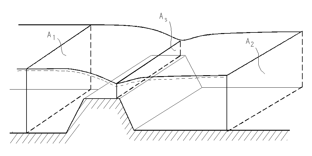
Figure: Cross-sectional flow areas at a structure showing entrance and exit velocity zones.

A minimum value for z₁ and z₂ can be specified in the HD parameter editor under the Default Values tab as ZetaMin. In the case \(A_{s} \to A_{1}\) the solution can become unstable (no friction) and specification of a minimum value of z_1,2, ensures a stable solution.

Expansion and contraction coefficients

As described in the previous section, flow through a structure is described according to:

\[ \Delta h = \zeta_{t}\frac{Q^{2}}{2gA^{2}} \]

Equation: Total headloss across the structure.

This equation z~ t~ describes the total headloss coefficient, which is composed of entrance (z₁) and exit (z₂) coefficients. For subcritical flow the coefficients are related to the input parameters z_in and z~out ~and the changes in velocity (v) and area (A):

\[ \zeta_{t} = \zeta_{1} + \zeta_{2} = \zeta_{in}\left(1 - \frac{v_{1}}{v_{s}}\right) + \zeta_{out}\left(1 - \frac{A_{s}}{A_{2}}\right)^{2} \]

Equation: Total loss coefficient, combining the inlet and outlet contributions.

For subcritical flow through a structure there is an upstream contraction and a downstream expansion, so equation the total loss coefficient, combining the inlet and outlet contributions works fine. When there is supercritical flow there is an upstream expansion and a downstream contraction. Thus if supercritical flow occurs then the loss coefficients are no longer valid. To accommodate supercritical flow, calculation of the of entrance (z₁) and exit (z₂) coefficients are expanded:

\[ \zeta_{1} = \begin{cases} \zeta_{in}\left(1 - \dfrac{v_{1}}{v_{s}}\right) & \text{for } v_{1} < v_{s} \\[1.5ex] \zeta_{in}\left(1 - \dfrac{A_{1}}{A_{s}}\right)^{2} & \text{for } v_{1} > v_{s} \end{cases} \]

Equation: Inlet headloss coefficient, depending on whether the inlet velocity is below or above the structure's characteristic velocity.

\[ \zeta_{2} = \begin{cases} \zeta_{out}\left(1 - \dfrac{v_{s}}{v_{2}}\right) & \text{for } v_{s} < v_{2} \\[1.5ex] \zeta_{out}\left(1 - \dfrac{A_{s}}{A_{2}}\right)^{2} & \text{for } v_{s} > v_{2} \end{cases} \]

Equation: Outlet headloss coefficient, depending on whether the structure's characteristic velocity is below or above the outlet velocity.

Care must be taken when selecting loss coefficients, particularly in situations where both subcritical and supercritical flow conditions occur. When flow conditions change from subcritical to supercritical (or the Froude number F_R becomes greater than 1), the loss coefficients z_in and z_out (specified in the Headloss Factors box) are modified:

• If F_R > 1 in upstream h-point then z_in = z_in / 2
• If F_R > 1 in downstream h-point then z_out = z_out / 2

Note that this adjustment is not made for bridge structures.

Determination of flow regime

Given the upstream and downstream water levels and the discharge, and assuming that these three values are compatible with each other, the type of flow can be determined as follows.

For zero flow the upstream and downstream water levels are both below the structure invert (crest level) and the flow regime is subcritical, or the flow direction is opposite valve regulation.

For differentiating between critical and drowned flow it is assumed, in the first instance, that the flow at the weir crest is critical.

The critical discharge is determined for broad crested weirs, special weirs and culverts via the tabulated QH-relation while it in case of structures with time dependent geometry is computed by critical flow iteration during the simulation. The pre-processed QH-relation for broad crested weirs are based on the assumption of a single structure, hence when the broad crested weir is a part of a composite structure the QH-relation is no longer valid. In this case the critical discharge is computed by iteration during the simulation. When special weirs and culverts are included in a composite structure it is assumed that the user defined QH-relations for critical flow takes the changed hydraulic conditions into account. When the upstream flow regime is supercritical, the QH-relations are also recalculated.

When a long culvert is a part of a composite structure, there is no critical discharge iteration i.e. the computed QH-relation is used to estimate the critical discharge. This approach is assumed valid as the structure area usually is much smaller than the upstream area i.e. \(A_{s} \ll A_{1}\) hence no need for iteration.

Critical flow occurs (for z₂ > 1) when the energy head at the crest is larger than the downstream energy head, viz.:

\[ h_{s} + \left(1 - \zeta_{2}\right)\frac{Q_{s}^{2}}{2gA_{s}^{2}} \geq h_{2} + \frac{Q_{s}^{2}}{2gA_{2}^{2}} \]

Equation: Energy condition for critical flow over a structure.

Critical flow occurs (for \(\zeta_{2} \leq 1\) and outflow headloss less or equal to 1) when the water level at the crest is larger than the downstream energy head:

\[ h_{s} \geq h_{2} + \frac{Q_{s}^{2}}{2gA_{2}^{2}} \]

Equation: Energy condition for critical flow at a weir or overflow structure.

If the flow is not critical, a submerged discharge iteration is performed and the submerged discharge is compared with the critical and the smallest is taken.

Discharge over specific structures

How the discharge and the discharge derivatives over specific structures for use in equation (A.2.39) are calculated is not presented in this document for all structures.

Section B.1 QH Relations Calculated for Culverts (p. 317) presents some details for culverts.

DELTA Coefficient

A forward centring of the \(\partial h/\partial x\) term in the numerical scheme has a dissipative influence which can be demonstrated using the Taylor-series. The forward centring is automatically introduced in MIKE 1D when the flow becomes supercritical in a particular section of a reach. Additionally, the centring can be specified by the user for subcritical flows through the centring coefficient DELTA (0.5 <d< 1).

Introducing the d value into the terms gives:

\[ \frac{\partial h}{\partial x} = \delta\frac{h_{j+1}^{n+1} - h_{j-1}^{n+1}}{\Delta 2x} + (1-\delta)\frac{h_{j+1}^{n} - h_{j-1}^{n}}{\Delta 2x} \]

Equation: Spatial derivative of h expanded as a Taylor series in the 6-point Abbot scheme.

Using a Taylor series up to the third derivative, these terms become:

\[ \frac{h_{j+1}^{n+1} - h_{j-1}^{n+1}}{\Delta 2x} = \frac{\delta}{\Delta 2x}\left[ h + \frac{1}{1!}\frac{\Delta 2x}{2}\frac{\partial h}{\partial x} + \frac{1}{2!}\left(\frac{\Delta 2x}{2}\right)^{2}\frac{\partial^{2} h}{\partial x^{2}} + \frac{1}{3!}\left(\frac{\Delta 2x}{2}\right)^{3}\frac{\partial^{3} h}{\partial x^{3}} - h + \frac{1}{1!}\frac{\Delta 2x}{2}\frac{\partial h}{\partial x} + \frac{1}{2!}\left(\frac{\Delta 2x}{2}\right)^{2}\frac{\partial^{2} h}{\partial x^{2}} + \frac{1}{3!}\left(\frac{\Delta 2x}{2}\right)^{3}\frac{\partial^{3} h}{\partial x^{3}} \right]_{j}^{n+1} = \delta\left[ \frac{\partial h}{\partial x} + \frac{\left(\Delta 2x\right)^{2}}{24}\frac{\partial^{3} h}{\partial x^{3}} \right] \]

Equation: Spatial derivative of h expanded as a Taylor series in the 6-point Abbot scheme.

Similarly for the last term:

\[ (1-\delta)\frac{h_{j+1}^{n} - h_{j-1}^{n}}{\Delta 2x} = (1-\delta)\left[\frac{\partial h}{\partial x} + \frac{\left(\Delta 2x\right)^{2}}{24}\frac{\partial^{3} h}{\partial x^{3}}\right]_{j}^{n} \]

Equation: The (1-delta)-weighted backward term of the spatial derivative, expanded as a Taylor series.

In this way the formulation of \(\partial h/\partial x\) in the spatial derivative of h expanded as a Taylor series in the 6-point Abbot scheme becomes (again using a Taylor series):

\[ \frac{\partial h}{\partial x} = \delta\left[ \frac{\partial h}{\partial x} + \frac{1}{1!}\frac{\Delta t}{2}\frac{\partial^{2} h}{\partial x \partial t} + \frac{1}{2!}\left(\frac{\Delta t}{2}\right)^{2}\frac{\partial^{3} h}{\partial x \partial t^{2}} \right]_{j}^{n+\frac{1}{2}} + (1-\delta)\left[ \frac{\partial h}{\partial x} - \frac{1}{1!}\frac{\Delta t}{2}\frac{\partial^{2} h}{\partial x \partial t} + \frac{1}{2!}\left(\frac{\Delta t}{2}\right)^{2}\frac{\partial^{3} h}{\partial x \partial t^{2}} \right]_{j}^{n+\frac{1}{2}} = \left.\frac{\partial h}{\partial x}\right|^{n+\frac{1}{2}} + (2\delta - 1)\frac{\Delta t}{2}\left.\frac{\partial^{2} h}{\partial x \partial t}\right|^{n+\frac{1}{2}} + \text{higher order terms} \]

Equation: The DELTA-weighted spatial derivative expanded as a Taylor series and simplified.

which represents a dissipative effect, when d>0.5, as the last term before the higher order terms becomes positive.

Also note that for d>0.5, the solution scheme is not second order, since 2d-1 not zero in equation (A.2.67).

Mass Balance

Theoretically, the applied computational scheme should ensure mass conservation in every case. In practical applications, the mass balance may be jeopardised in a number of situations, such as:

• Relatively sharp changes of storage width due to rapid changes of water depth or a sharp change of cross section shape with depth. This may be e.g. the case at relatively small depths in circular pipes and in cross sections with flow bank zones.
• Sharp changes in surface area of basins
• Surcharge of manholes

The scale of the problem is usually related to the length of the simulation time step.

Improved Continuity Balance for Links

Urban (MIKE+)

This section applies to MIKE+ type setups only.

While solving the continuity equation:

\[ \frac{\partial q}{\partial x} + b_{s}\frac{\partial h}{\partial t} = q_{in} \]

Equation: The continuity equation, with the storage width bs introduced.

the storage width, b_s, is in the first iteration approximated at time n, and in subsequent iterations at time n+½. In situations where only one iteration is performed, as is typically the case in MIKE+ type setups, the approximation can imply a significant amount of water being generated or disappearing, giving a significant mass balance error.

A Taylor expansion of the storage width can greatly improve on the mass balance error. Expanding the storage width around time n gives:

\[ b_{s}^{n+\delta} = b_{s}^{n} + \delta\Delta t\frac{\partial b}{\partial h}\frac{\partial h}{\partial t} \]

Equation: Storage width at the new time level, from a first-order Taylor expansion.

Isolating and inserting the \(\partial h/\partial t\) term from the continuity equation:

\[ b_{s}^{n+\delta} = b_{s}^{n} + \delta\frac{\Delta t}{b_{s}}\frac{\partial b}{\partial h}\left(-\frac{\partial q}{\partial x} + q_{in}\right) \]

Equation: Storage width at the new time level, substituting the continuity equation for the time derivative of water level.

Rearrange to get the contribution as a correction term:

\[ b_{s}^{n+\delta} = b_{s}^{n} \cdot \left(1 + \delta\frac{\Delta t}{\left(b_{s}^{n}\right)^{2}}\left.\frac{\partial b}{\partial h}\right|^{n}\left(-\left.\frac{\partial q}{\partial x}\right|^{n} + q_{in}\right)\right) \]

Equation: Storage width at the new time level, rearranged into an explicit update formula.

This modification is applicable only for cross sections with relatively smooth changes of the storage width. As the width for arbitrary cross sections can vary in very unpredictable ways, the correction is only applied to the standard predefined cross sections.

It should be noted that errors in the mass balance occur when changes in storage width are significant as the water level changes. Since cross sections typically become narrow at the bottom, errors in the mass balance can sometimes be controlled by adjusting the minimum water depth (i.e. make sure that reaches do not run dry). See the user manual for information about how to control the minimum water depth.

Some Special Techniques

Expanding node covers (Surface flooding)

This technique is used to simulate manholes and basins that flood surrounding surfaces, with the water assumed to re-enter the collection system network after the flooding event.

If the water level in an open manhole or a basin reaches ground level, an artificial inundation basin is inserted above the node. The surface area of this artificial basin is gradually increased from the top of the manhole or the basin, thus simulating the surface inundation. When the outflow from the node becomes greater than the inflow, the water stored in the inundation basin re-enters the system.

The inundation basin is simulated by assuming an expansion from the manhole or basin. The rate of expansion is controlled by a parameter specified in the MIKE 1D engine configuration tab. Different parameter values are applied to manholes and basins. The manhole expansion parameter is called, "Manhole cover expansion coefficient", and the default value is 1000. The basin parameter is called, "Basin cover expansion coefficient", and the default value is 1. The basin parameter also controls the expansion of inundation basin for soakaways. The effect of the default values is that the manhole inundation basin increases to 1000 times the manhole area, while the basin area does not become larger than the top of the basin geometry curve.

Expansion is assumed to take place over a vertical distance of 1 metre. For manholes, the starting elevation of the expansion is specified in the MIKE 1D engine configuration tab, using the parameter, "Node cover start level. The default value is 0.25m below ground level. For basins and soakaways, the expansion begins at the top of the geometry curve.

Mathematically, the expanding cover enters the node equations (see Section A.2.2) only through the calculation of the surface area in the node. For the expanding manhole cover with default expansion coefficient, the surface area is

\[ A_{fl} = \text{Min}\left(A_{fl,node} \cdot e^{7\left(H - H_{gl} - 0.25\right)}, 1000A_{fl,node}\right) \]

Equation: Flow area for an expanding node cover, capped at a minimum and growing exponentially with water level above ground.

where \(A_{fl,node}\) is the surface area just below the cover and \(H_{gl}\) is the ground level.

When the water level in the node increases and is above ground level, it is assumed that during a time step, the surface area in the basin is calculated using the water level from the start of the time step. A situation like this is shown in the simulation of surface flooding. If the water level passes through the transition region between the actual manhole or structure and the artificial basin. This leads to generation of water. In the simulation of surface flooding the shaded area illustrates the generated volume of water.

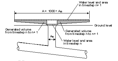
Figure: Simulation of surface flooding.

Figure: Surface flooding showing generated water volume at manhole or basin expansion.

When the increase of the water level during a time step is relatively small, then the generated water volume is negligible. If the water level is changing rapidly, the generated volume of water is important. Therefore, MIKE 1D will calculate the difference in water volume and correct the mass balance accordingly in the following time step.

Sealed Nodes

Manholes and basins can be defined as 'sealed'. If they are defined as sealed, then water will not flow onto the surface. Instead, the water enters a narrow slot comparable to the slot on closed cross sections.

The narrow slot is simulated with a sealed cover that gradually contracts to a slot with a diameter of \(w_{slot}^{2}\) times the node diameter, where \(w_{slot}\) is the width of a slot cover at infinite height. The contraction happens gradually, starting 0.25m (default value) below ground level.

Mathematically, the sealed cover enters the node equations (see Section A.2.2) only through the calculation of the surface area in the node. For a sealed cover the surface area is

\[ A_{fl} = A_{fl,node}\left[\left(1 - w_{slot}\right)e^{\frac{6\left(H - H_{gl} - 0.25\right)}{D}} - w_{slot}\right] \]

Equation: Flow area for a sealed node cover, contracting from a narrow slot as water level rises.

where D is the diameter of the node just below the cover.

Spilling Nodes

Any manhole or basin can be defined as 'spilling'. If the water level in a node defined as a spilling node reaches the ground level, the water will start spilling irreversibly out of the system. The flow will be computed using the free overflow formula, according to the following:

\[ \text{for } H \leq \left(H_{gl} + \Delta P\right): \quad Q_{spill} = 0; \qquad \text{for } H > \left(H_{gl} + \Delta P\right): \quad Q_{spill} = \text{Relative Weir Coefficient} \cdot 0.63 \cdot B \cdot \sqrt{2g} \cdot \left(H - \left(H_{gl} + \Delta P\right)\right)^{3/2} \]

Equation: Spill discharge from a spilling cover, zero below the buffer pressure level and a weir formula above it.

where:

• Q_spill — the spill discharge [m³/s]
• B — a conceptual spill width [m]
• H~~ — the water level in the manhole [m]
• H_gl — the ground level in the manhole [m]
• DP — the “Buffer Pressure Level” for the spill [m]
• g — the acceleration of gravity [ms^-2) RelativeWeirCoefficient = the linear scaling coefficient for the spill.

The level (i.e. head) at which the spill starts can be controlled by optionally specifying the 'Buffer Pressure Level' as a relative elevation above (or below) the ground surface (default value = 0).

For circular manholes, the spill width B equals to 1.5 times the manhole diameter for the water level H = H_gl+DP. With increasing water level, the spill width B increases, following the same functional relation as used for the area above expanding nodes (i.e. increases exponentially to approximately Max. 1000 times the manhole diameter), see Section A.4.1.

The spilling capacity of a spilling manhole can be controlled by specifying the Relative Weir Coefficient (default value = 1).

Displaceable covers

A manhole or basin can have a cover that is displaced by pressure. Before displacement, the cover functions like a sealed cover. After displacement, the cover is like a spilling cover in that water flowing out of the cover is assumed to exit the system.

Displacement is controlled by a pressure-fraction table that determines how much the cover will be displaced by pressure in the node. The displacement fraction, f, must be defined in the interval [0;1] where f=0 means no displacement/sealed cover, and f=1 means cover is completely removed and spilling occurs at full orifice area. In the MIKE+ GUI, the fraction is defined using a percentage scale. Displacement cannot decrease with increasing pressure.

Discharge through a displaced cover may resemble orifice or weir flow, depending on the extent of displacement. A partially displaced cover is more likely to exhibit orifice flow, while flow out of a fully displaced cover is better simulated using a weir assumption. During each time step, MIKE 1D estimates flow out of the node using both assumptions and then applies the lesser of the two estimates.

The weir flow estimate is made using an approach like that used for a spilling cover.

\[ Q_{weir} = 0.63BC_{w}\Delta H\sqrt{2g\Delta H} \]

Equation: Discharge over a spilling cover, weir formula.

where

• Q_weir — discharge estimated with weir assumption [m³/s]
• C_w — linear scaling coefficient (spill coefficient) DH = H - H_gl, where H is the water level in the node and H_gl is the ground level.

The conceptual spill width, B, is related to the displacement fraction f as follows:

\[ B = 1.5e^{3.5\Delta H}d_{f} \]

Equation: Width of the spilling cover crest, growing exponentially with head above the crest.

where the orifice diameter, d_f, is given as

\[ d_{f} = \sqrt{Af4/\pi} \]

Equation: Diameter-equivalent width factor used in the spilling cover geometry.

with A being the area of the manhole or basin when it is fully open.

The orifice flow estimate assumes that the pressure head is converted to flow out of the orifice after accounting for a contraction loss coefficient.

\[ Q_{orifice} = C_{orifice}Af\sqrt{2g\Delta H} \]

Equation: Discharge over a spilling cover, orifice formula.

where

Q_orifice = discharge estimated using orifice assumption [m³/s]

C_orifice=1 - q (contraction coefficient)

q = 0.5 (1 - Af)

For stability reasons, MIKE 1D constrains the rate at which a cover can be displaced. The parameter "Maximum manhole displacement rate" controls the rate at which the displacement fraction changes per second. The parameter can be modified in the MIKE 1D engine configuration window.

Dry Conduits and Numerical Water

Urban (MIKE+)

This section applies to MIKE+ type setups, where a bottom slot is not applied.

The 1D engine will not allow the water depth in reaches to become zero. If parts of the network are close to drying out, then the 1D engine maintains a minimum water depth in those parts, that by default is 5‰ of the characteristic dimension of the conduit (diameter for circular pipes), or Max. 5 mm. This is necessary in order to maintain numerical stability in the solution of the flow equations.

This correction practically means artificial generation of water, i.e. some water volume is added to the system. As a consequence of that, the continuity status report shown does not give a fair impression of the accuracy of the simulation. The amount of water added due to drying out of reaches is normally referred to as numerical water.

Bottom Slots

During low flow conditions (the local water depth is less than DELH, where DELH is a user specified parameter) a bottom slot can be introduced into the computations. The slot starts DELH over the bottom and extends 5 times DELH below the cross section bottom, see the schematic diagram showing the geometry of a bottom slot.

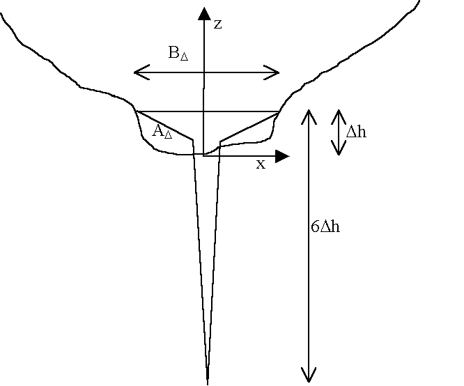
Figure: Geometry of bottom slots extending below cross-section bottom during low flow.

Classical bottom slot

The classical bottom slot description is given by

\[ B = \frac{\sqrt{z + 5\Delta h}}{\sqrt{6\Delta h}}B_{\Delta} \]

Equation: Width of the narrow slot cover as a function of height above the node bottom.

where z is the water depth with origin at the bed (lowest cross section point), i.e. it can be negative. It has the area

\[ A(z) = \int_{-5\Delta h}^{z}B(z)\,dz = \frac{2\left(z + 5\Delta h\right)^{3/2}}{3\sqrt{6\Delta h}}B_{\Delta} \]

Equation: Cross-sectional area of the narrow slot cover, integrated from the width function.

Area preserving bottom slot

As an alternative the slot may given a geometry such that the cross sectional area at the top of the slot matches exactly that of the cross section at that level, i.e. the area varies continuously across the level at which the slot is introduced.

The width B of the slot is given by the following expression

\[ B = \begin{cases} \dfrac{B_{\Delta}\left(\Delta h - z_{0}\right)}{\Delta h\left(z_{0} + 5\Delta h\right)}\left(z + 5\Delta h\right) & \text{for } -5\Delta h \leq z \leq z_{0} \\[1.5ex] -\dfrac{B_{\Delta} z_{0}}{\Delta h\left(z_{0} - \Delta h\right)}\left(z - \Delta h\right) + B_{\Delta} & \text{for } z_{0} < z \leq \Delta h \end{cases} \]

Equation: Width of the narrow slot cover as a function of height above the node bottom.

where

A_Dis the cross sectional area Dh above the bottom

B_Dis the channel width at the same level.

Dh is the user defined DELH.

and

\[ z_{0} = \Delta h - \frac{2A_{\Delta}}{7B_{\Delta}} \]

Equation: Reference elevation used in the narrow slot cover geometry.

River (MIKE 11 / MIKE HYDRO)

The choice of slot description is set in the MIKE11.ini file through the variable AREA_PRESERVING_SLOT. The default setting is the classical description e.g. the width of the narrow slot cover as a function of height above the node bottom.

Constant AWR Top Slot

The constant ARW top slot is intended for closed cross sections and are vital when pressurised flow are considered, see Section 4.2.

When water enters the slot, water can still flow into the reach section, but the flow area of the cross section (and thereby the volume of water in the reach) stays the same, i.e., water disappears in the process. The water disappears when the water level rises and appears again when the water level is falls.

The argument for keeping the area constant is that the momentum term in the momentum equation contains a \(Q^{2}/A\) term. If \(A\) is increasing, the momentum will drop, and thereby the velocity. The velocity should not decrease when the pipe gets under pressure.

B Appendix

Structure Module

QH Relations Calculated for Culverts

This appendix presents details of how the discharge is calculated for culverts where the QH relations are provided by the 1D engine. These details expand on the presentation of Section 6.7.2.

Loss Coefficients

The contraction, expansion, friction and bend loss coefficients, and the critical flow correction coefficient are described as follows.

Entrance loss

The contraction loss coefficient, z₁, is a function of the inflow loss coefficient, z_in, the culvert inflow cross section area, _{\(A_{s_{1}}\)}, and the inflow river cross section area, A₁. Typically, z_in is set to 0.5.

\[ \zeta_{1} = \zeta_{in}\left(1 - \frac{A_{s_{1}}}{A_{1}}\right) \]

Equation: Inlet headloss coefficient, depending on the ratio of the structure's surface area to the inlet area.

Expansion loss

The expansion loss coefficient, z₂, is a function of the outflow loss coefficient, z_out, and the culvert outflow cross section area, _{\(A_{s_{2}}\)}, and the outflow river cross section area, A₂. Typically z_out is set to 1.0.

\[ \zeta_{1} = \zeta_{out}\left(1 - \frac{A_{s_{2}}}{A_{2}}\right)^{2} \]

Equation: Outlet headloss coefficient, depending on the ratio of the structure's surface area to the outlet area.

River (MIKE 11 / MIKE HYDRO)

In MIKE 11, the outflow loss coefficient, z_out, is specified in the Network editor ® structures ® culverts in the Headloss Factor Box.

Friction loss

The friction loss coefficient is calculated using the Manning formula, i.e.:

\[ \zeta_{f} = \frac{2gLn^{2}}{R^{4/3}} \]

Equation: Friction loss coefficient, Manning formulation.

where, L is the culvert length, n is Manning's coefficient and R is the mean hydraulic radius along the culvert. The Manning's n value depends on the interior surface of the culvert. Tables of values can be found in open channel or closed conduit hydraulics references such as (² and ³). For a concrete culvert n would typically range from 0.011 to 0.017.

Bend and other losses

The bend loss coefficient, z_b, is provided for situations where headlosses other than from the above occur, for example bends, damaged culverts, trapped debris. The headloss due to z_b is defined in the total headloss given below. For straight culverts in good condition a value of zero would apply.

Total headloss through culvert

The total headloss, DH_loss, through the culvert is given by

\[ \Delta H_{loss} = \frac{Q^{2}}{2g}\left(\frac{\zeta_{1}}{A_{s_{1}}^{2}} + \frac{\zeta_{f} + \zeta_{b}}{A_{s_{a}}^{2}} + \frac{\zeta_{2}}{A_{s_{2}}^{2}}\right) \]

Equation: Total headloss through a culvert from entrance, friction, and exit energy losses.

where, \(A_{s_{a}}\) is the mean cross section area along the length of the culvert, and Q is the discharge.

Critical flow correction factor

The critical and orifice flows are multiplied by the critical flow correction factor, a_c, see Section 6.1 General Flow Conditions (p. 95), for more details. Typically a value of 1.0 is used.

River (MIKE 11 / MIKE HYDRO)

In MIKE 11, the critical flow correction factor, a_c, is specified in the Network editor ® structures ® culverts in the Headloss Factor Box as the Free Overflow Headloss Factor.

Discharge for Critical Inflow or Outflow

In the case of either critical inflow or outflow being critical the discharge, Q_c, for a given critical depth is calculated as:

\[ Q_{c} = \alpha_{c}A_{c}\sqrt{g\frac{A_{c}}{T}} \]

Equation: Critical discharge at a cross section.

where, A_c is the critical flow area and T is the flow width at the water surface.

Condition for Critical Inflow

Critical flow at the inflow to the culvert inlet occurs when the geometrical slope, S₀, exceeds the critical flow slope, S_c, as defined by:

\[ S_{0} = \frac{z_{inv_{1}} - z_{inv_{2}}}{L} \quad \text{and} \quad S_{c} = \left(\frac{Q_{c}n}{A_{c}R_{c}^{2/3}}\right)^{2} \]

Equation: Bed slope and critical slope used to determine whether the flow is sub- or super-critical.

where, \(z_{inv_{1}}\) and \(z_{inv_{2}}\)are the inflow and outflow invert levels of the culvert, and R_c is the hydraulic radius at critical flow.

For the calculation of h₁, the inflow water depth is taken as the critical depth. The friction losses and bend losses have no effect on the discharge for this flow condition.

Condition for Critical Outflow

Critical flow at the outflow to the culvert outlet occurs when S₀ is less than S_c.

Before the calculation of h₁ can proceed, it is necessary to determine the inflow water depth. A standard backwater analysis using a fine increment in water depth is used starting with the critical flow depth at the outflow end and working its way upstream. The bend losses, if any, are applied at the mid-point along the length of the culvert.

In the situation of the culvert section becoming full (i.e., submerged inflow), the friction slope becomes constant and the backwater analysis adjusts accordingly.

The upstream water level is calculated based on the inflow water depth in the culvert using the iterative procedure described in Section 6.7.2.

Orifice Flow at Inflow

Orifice flow occurs in short or steep culverts (the flow descriptions(e)). Culverts in which this flow condition occurs are sometimes referred to as “hydraulically short” (²). The flow is similar to that which occurs under a sluice gate. The discharge is calculated as:

\[ Q_{0} = \alpha_{c}C_{0}A_{full}\sqrt{2g\left(H_{1} - z_{inv_{1}}\right)} \]

Equation: Initial discharge at a free outfall boundary.

where, C₀ is the coefficient of discharge, H₁ is the inflow energy head in the river, \(z_{inv_{1}}\)is the inflow invert level, and A_full is the full cross section area of the culvert.

River (MIKE 11 / MIKE HYDRO)

In MIKE11, the facility to manually specify C₀ as a function of y₁/D (y₁=h₁-\(z_{inv_{1}}\) and D = culvert depth) has been provided in the network editor ® structures ® culverts ® Flow conditions under the Orifice Flow Conditions Tab.

It is anticipated that in most conditions it will be unnecessary to provide C₀ as a default is provided (discussed below). However, it does provide the flexibility to model a “hydraulically short” culvert, or a sluice gate (zero length) in detail if sufficient information on the discharge coefficient is available. (²) provides a detailed analysis and tables of discharge coefficients for orifice flow and other flow conditions.

If no values for C₀ are specified, a value of 0.65 at y₁/D equal to 5.0 is adopted. When y₁/D is greater than 5.0, C₀ remains constant at 0.65, while below 5.0 a linear interpolation is made with the C₀ value calculated automatically.

A value for C₀ is automatically calculated at the point of inflow submergence if the flow condition is inflow critical. This allows a smooth transition to occur between the two flow conditions. The point of inflow submergence is nominally adopted as 95% of the full culvert flow area. The calculated C₀ value is shown in the first row of the C₀ vs y/D tables.

Full Culvert Flow with Free Outflow

The complement to orifice flow at the inflow is when the culvert is defined as “hydraulically long”, i.e., the culvert is flowing full with a free outflow (the flow descriptions (f)). In this case the discharge, Q_p is calculated as:

\[ Q_{p} = A_{full}\sqrt{\frac{2g\left(H_{1} - z_{obv_{2}}\right)}{\zeta_{1} + \zeta_{f} + \zeta_{b} + 1}} \]

Equation: Discharge at a free outfall boundary, including the headloss coefficients along the approach.

where H₁ is the inflow energy head level in the river and \(z_{obv_{2}}\)is the outflow soffit level (i.e. invert plus culvert depth).

The outflow energy head level in the above equation has been set to that at the outflow soffit by assuming atmospheric pressure occurs there. This assumption is compatible with the critical outflow flow condition at the point of the outflow becoming submerged as the discharge equations are the same if z₂ is equal to 1.0. This is important for the transition between upstream and downstream controlled flow conditions as discussed later.

Downstream Controlled Flow (Submerged Flow)

In the case of a downstream controlled flow the computation is complicated because of the influence of all three cross section areas along the culvert, \(A_{s_{1}}\), \(A_{s_{a}}\) and \(A_{s_{2}}\), and the mean hydraulic radius, R. The situation is further complicated in the case where the culvert outflow is close to critical flow conditions as the water surface profile throughout the culvert under these conditions is very non-linear.

Partially Full Inflow and Outflow

An iterative procedure is used to determine \(A_{s_{1}}\), \(A_{s_{a}}\), \(A_{s_{2}}\) and R. The iterations are made on the water levels in the culvert at the upstream and downstream ends, Equations (B.1.9a) and (B.1.9b), from which \(A_{s_{1}}\) and \(A_{s_{2}}\) are calculated. For \(A_{s_{a}}\) and R, a linear interpolation of the water level at the culvert mid-point is initially used.

\[ h_{s_{1}} = H_{1} - \frac{\left(1 + \zeta_{1}\right)\left(H_{1} - H_{2}\right)}{C_{a_{s}}A_{s_{1}}^{2}} \]

Equation: Water level at the inlet side of a headloss structure.

\[ h_{s_{2}} = H_{2} - \frac{\left(1 - \zeta_{2}\right)\left(H_{1} - H_{2}\right)}{C_{a_{s}}A_{s_{2}}^{2}} \]

Equation: Water level at the outlet side of a headloss structure.

where

\[ C_{a_{s}} = \frac{\zeta_{1}}{A_{s_{1}}^{2}} + \frac{\left(\zeta_{f} + \zeta_{b}\right)}{A_{s_{a}}^{2}} + \frac{\zeta_{2}}{A_{s_{2}}^{2}} \]

Equation: Combined headloss coefficient across the structure.

\(h_{s_{1}}\)and \(h_{s_{2}}\)are the water levels in the culvert at the inflow and outflow ends, while H₁ and H₂ are the inflow and outflow energy head levels in the river.

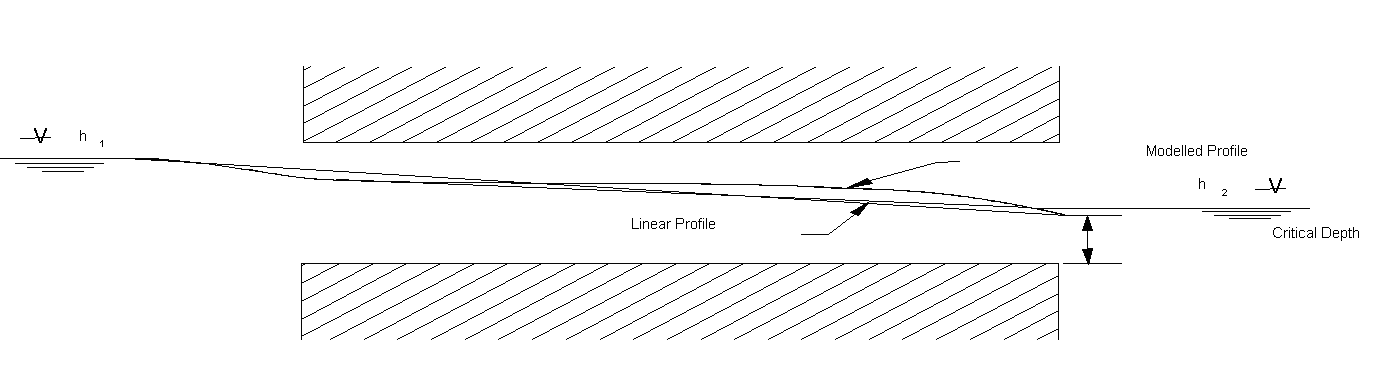
Figure: Nonlinear water surface profile showing energy levels at culvert inflow and outflow.

When the outflow is close to a critical flow state the water surface profile is highly non-linear, and the friction losses calculated from a linear interpolation will be too high (the water surface profile in the culvert at the inflow and outflow ends when the). To overcome this problem without using a computationally intensive backwater analysis in each iteration, a comparison is made with the friction losses calculated from the backwater analysis for critical outflow, see above. In the case of the losses from the backwater analysis being lower, \(C_{a_{s}}\) is calculated as:

\[ C_{a_{s}} = \frac{2g}{Q_{c}^{2}}\left(H_{1} - h_{c} - \frac{Q_{c}^{2}}{2gA_{c}^{2}}\right) + \frac{\zeta_{2}}{A_{s_{2}}^{2}} \]

Equation: Combined headloss coefficient, expressed through the critical flow condition.

where the subscript _c refers to the critical flow conditions based on h₁. This also ensures a smooth transition between the outflow critical condition and submerged flow provided that z₂ is less than or equal to 1.0.

The iterative procedure typically takes two to three iterations to converge. If the upstream and downstream water levels are changing rapidly more iterations are usually necessary with the number rarely exceeding ten. The maximum number of iterations is controlled by the Inter1Max variable.

River (MIKE 11 / MIKE HYDRO)

In MIKE 11, the Inter1Max variable can be edited in the HD parameter editor ®Default values.

Submerged Inflow and Partially Full Outflow

This flow condition typically occurs when the culvert slope is adverse to the water surface slope as shown in the flow descriptions(h).

The iteration procedure described above is used except that the mean cross section area is adjusted according to:

\[ A_{s_{a}} = \frac{L_{full}}{L}A_{full} + \left(1 - \frac{L_{full}}{L}\right)\frac{A_{full} + A_{s_{2}}}{2} \]

Equation: Effective storage area at a structure, interpolated between the full node area and the outlet area.

where L_full is the length of the culvert which is following full and L is the total length.

A similar adjustment is made to the mean hydraulic radius.

Partially Full Inflow and Submerged Outflow

This flow condition occurs in sloping culverts as illustrated in the flow descriptions(i). A similar procedure to that described in “Submerged Inflow and Partially Full Outflow” above is used.

Fully Submerged

Where the culvert is fully submerged (the flow descriptions(j)) the cross section areas and hydraulic radius are equal to those when the culvert is full.

Transition between Upstream and Downstream Control

Whether the flow is upstream or downstream controlled is best based on a single criterion. Using a single criterion is preferable for stability reasons and for a smooth transition between flow conditions.

Analysis of the formulations described above, assuming that z₂ is less than or equal to 1.0, gives the following conclusions:

• In the case of either inflow or outflow being critical, then if H₂ is below the critical water level, h_c, the flow will be critical. If H₂ is greater than h_c then the flow can be either critical or downstream controlled. The level at which the flow becomes downstream controlled is dependent on the magnitude of z₂. If z₂ is equal to 1.0 the change to or from submerged flow will be at H₂ equal to h_c. For z₂ less than 1.0, which is normally the case, downstream controlled flow will occur at some point above h_c.
• Similarly, the same scenario can be shown to occur for full culvert flow and orifice flow versus fully submerged flow where h_c is taken as the outflow soffit (invert plus culvert depth).

This leads to the following criteria for selecting between upstream and downstream flow controls:

• If H₂ is less than either h_c at outflow (critical inflow or outflow) or the downstream soffit (orifice or full culvert flow) then the flow is upstream controlled, otherwise the flow condition which gives the lower discharge is selected

In the case of critical inflow, H₂ should be taken as that immediately past the point of critical flow (i.e., at the inlet of the culvert). However, for culverts of non-zero length and/or non-zero bend loss, the energy headlosses through the culvert are not known and the more conservative approach of using h_c at the outflow must be taken. A similar situation applies in the case of orifice flow.

C APPENDIX

Misc

2D Mapping, Flood Maps

River (MIKE 11 / MIKE HYDRO)

Outlined below is the interpolation routine used to generate the various two dimensional maps. These maps can currently only be setup when running a MIKE 11 setup

The mapping of water levels, water depths, velocities and advection dispersion components from the one-dimensional results to two-dimensional maps are done through a number of steps:

• Interpolation of horizontal 2D cross section end point coordinates at all digitised points and all interpolated water level points.
• Mapping between the horizontal 2D (x,y) coordinate an the river coordinate system (chainage and transversal distance from centre of river).
• Linear interpolation of results in the river coordinate system can then be mapped to the 2D coordinate system.

All cells in the 2D grid can spatially interpolate a bed level, water level etc. by using the interpolation and mapping routines.

Interpolation of Cross Section Coordinates

The network consists of digitised points and cross sections, and the two are related by their chainage value. A typical network can be seen in the typical reach with digitised points and cross sections. The circles illustrate the digitised points. The cross sections are shown as the full drawn lines.

Figure: Flood map network showing digitized points and cross-section locations with chainage.

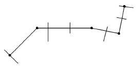
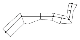
The first step is to obtain a 2D envelope of the river system that follows the digitised points, as in the river 2D envelope

Figure: 2D envelope of the river system following digitized points for flood mapping.

This is obtained by considering the river as a straight line as in the reach from 1D river coordinates point of view. Dashed lines are interpolated, which is called the river coordinate system. In this river coordinate system, the left/right river width can be interpolated at the digitised points and the interpolated water level points by linear interpolation. The interpolated cross section positions are indicated by dashed lines in the plot.

Figure: Interpolated water levels and cross-section positions with dashed lines indicating interpolation.

The interpolated widths are used at the digitised points and the interpolated water level points to obtain the 2D horizontal (x,y) coordinates of the river sides, and straight lines between the river side coordinates down the river are used to form the 2D envelope.

Mapping between 2D and 1D Coordinate Systems

Figure: Mapping of xy coordinates to local uv coordinates for river flow mapping.

The reach is split into a number of segments, bounded by either a digitised point or an interpolated water level point. Each segment has cross section end point coordinates at each end. An actual cross section need not exist at the end of the segments, but further up/down the river. Such a segment is termed a mapping box. the mapping from (x,y) to river system coordinates shows a mapping box in grey and bounded by the dashed lines. In this case cross sections are defined further up/down of the mapping box, indicated by full drawn lines. For each of these mapping boxes a set of local (u,v) coordinate systems are introduced on each side of the river centre line (lowest point line), the mapping from (x,y) to river system coordinates shows one. The (x,y) point in the figure marked with a circle is mapped to the local (u,v) coordinates (0,5;0,5). From this local coordinates it is possible to calculate the river coordinates, chainage and width.

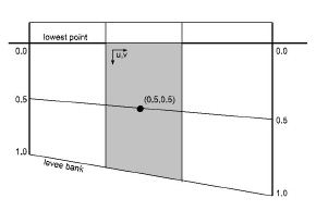
Figure: Mapping from (x,y) to river system coordinates.

Figure: Multiple local uv mappings at river bank showing different coordinate systems in mapping boxes.

For a given (x,y) coordinate, a value is calculated by first mapping the (x,y) coordinate to local (u,v) coordinate system, calculate the river coordinates, and then linearly interpolate the value in the river coordinate system.

When left and/or right bank markers are set, the local mapping needs to take place between each marker line, as in the mapping from (x,y) to river system coordinates when bank markers are specified, hence up to 4 local different (u,v) mappings can take place within a mapping box. Note especially that the relative local river v coordinate differs in each end of the mapping box.

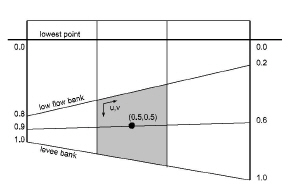
Figure: Degenerate mapping boxes with intersecting sides showing overlapping regions excluded from mapping.

In case one of the cross sections does not define the bank marker, the quadrilateral (u,v) mapping degenerates to a triangle.

In some cases the cross sections lines in each end of a mapping box intersects. An example is shown in the mapping box with intersection cross section lines. The grey B* part is ignored, where the mapping box B between point 2 and 3 has intersecting sides. The grey area B* is overlapping both the A, B and C mapping box. The B* part of the B mapping box is disregarded.

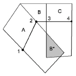
Figure: Mapping box with intersection cross section lines. The grey B* part is ignored in the B mapping box.

Linear Interpolation of Results

The interpolation of results at a given grid cell in the 2D map grid depends on the type of result:

• Water levels and concentrations are interpolated between nearest h-points based on the chainage coordinate of the grid cell. Values are only shown if the water level is above the local bed level at the grid cell.
• Water depth is determined as the water level minus the bed level, and will only be shown if the value is positive.
• Velocity is interpolated between the nearest h-points, and is only shown if the water level is above the local bed level at the grid cell.

In all cases results are only provided if the cross sections are open cross sections. Closed cross sections are assumed not to contribute to the map results.

Calculating the Local Velocity Profile in a Grid Point

The velocity distribution in a cross section is assumed to be uniform over the depth and vary as the conveyance in the transversal direction.

The total conveyance K is in this context defined as

\[ K(t) = \int_{0}^{b_{s}(t)}d\left(x,t\right)^{5/3}M(x)\,dx \]

Equation: Total conveyance of a cross section, expressed as the integral of the conveyance density over the wetted width.

where the integration takes place along the cross section profile that is wet, \(b_{s}\) is the width of the cross section, d is the local water depth along the cross section and M is the Manning resistance number. The water depth varies over the cross section, and Manning’s resistance number can also vary over the cross section, but it need not do so. For the Chezy description, the 5/3 is replaced with 3/2 and M is replaced by the Chezy number C

The velocity for a given point in the cross section is defined by

\[ v(x,t) = \frac{q(t)}{K(t)} \cdot M(x) \cdot d(x,t)^{2/3} \]

Equation: Velocity distribution across the cross section width, from the conveyance density.

where the q is the interpolated discharge at the cross section. For the Chezy formulation the M is again replaced by C and the 2/3 s replaced by 1/2.

Hereby a value for the velocity can be found at every point along the cross section, and the velocity in intermediate grid cell points in a mapping box are found by linear interpolation.

For a cross section that does not have raw data defined, or where the cross section is not fully open, above formulation can not take place or is not valid. Instead the velocity result will be just a simple average over the entire cross section and not vary along the cross section.

\[ v(t) = \frac{q(t)}{A_{fl}(h(t))} \]

Equation: Cross-sectional average velocity.

D APPENDIX

Default Values in MIKE 11 and MIKE+

MIKE 11 Default Values

River (MIKE 11 / MIKE HYDRO)

In MIKE 11, a number of parameters can be supplied in the “Default Values” tab of the HD Parameters file. The subset of the parameters that are supported by MIKE 1D are described here.

ALPHA Coefficient

This is the velocity distribution coefficient used in the momentum equation, see SectionA.2 Solving the Saint-Venant Equations (p. 285). The default value is 1.0.

DELH Coefficient

DELH controls the depth and top elevation of the slot in low flow conditions. The slot is inserted at height DELH above the river bottom and extends to a depth 5 x DELH below this level. See Section A.4.6.2 Area preserving bottom slot (p. 312). The default value is 0.1 m.

DELHS Coefficient

DELHS is used to prevent instabilities arising when the water surface gradient across a structure changes sign, see Chapter 6 on structures. It specifies the water level difference across a weir below which the flow description is linearised to obtain a stable solution. The default value is 0.01 m.

DELTA Coefficient

A forward centring of the ∂h/∂x-term in the numerical scheme has a dissipating influence which can be demonstrated using the Taylor-series, see Section A.2.5 DELTA Coefficient (p. 303). The forward centring is automatically introduced into MIKE 11 where the flow has become supercritical.

The dissipative influence of the forward centring can be controlled by the user for sub-critical flows through the coefficient DELTA (0.5 <= d <= 1). A value of 0.5 (the default) has no dissipative effect, while a value of 1.0 has maximum influence.

Changing the value of DELTA from its default value should only be carried out when “short term” fluctuations are unimportant, as in the case of a wave with a period of several days or longer.

FroudeExp

MIKE 1D offers two alternatives to the suppression of the convective terms in the Momentum equation for supercritical flow. If a negative value is entered for FroudeExp or FroudeMax (see below) then the default suppression is applied. FroudeExp is the exponential coefficient in the alternative suppression term.

FroudeMax

FroudeMax is the value at which the suppression sets in. As above if this is set to a negative value the default suppression is applied.

Inter1Max

This coefficient gives the maximum number of iterations permitted per time step to obtain a solution at a structure, see Section 6 Structures (p. 95). The default value is 10.

NoITER

NoITER specifies the number of iterations used in each time step to obtain a solution. The default value is 1. See Section A.2 Solving the Saint-Venant Equations (p. 285).

THETA

THETA is used in the discretisation of the momentum equation in the Fully Dynamic Wave Approximation (it is not used in the Fully Dynamic Higher Order Approximation). It can be used to dampen the instabilities from rapidly varying discharges and discharge reversals. The default value is 1.0 See Section Fully dynamic, MIKE 11 (p. 290).

Zeta Min

The headloss over structures is calculated according to Section 6 Structures (p. 95). The user has the option of specifying a minimum headloss, Zeta Min which is the lowest acceptable value of the sum of the headloss factors.

MIKE11.INI File Settings

River (MIKE 11 / MIKE HYDRO)

The Mike11.ini file contains settings for MIKE 1D. The file is loaded in the MIKE 11 bridge, and as such the settings in Mike11.ini are only relevant when MIKE 1D is running MIKE 11 setups.

MIKE 11 HD Settings

The section describes settings that are relevant for hydrodynamic calculations.

WL_EXCEEDANCE_FACTOR

WL_EXCEEDANCE_FACTOR defines when the calculation fails if water exceeds the banks of an open cross section. The maximum allowed water in an open cross section is WL_EXCEEDANCE_FACTOR times the height of the cross section. By default, open cross sections are extended upward with vertical walls in the full width of the cross section.

Allowed values: Any positive value.

Default value: 4.0.

MAX_GATE_ITERATIONS

MAX_GATE_ITERATIONS defines the maximum allowed number of iterations during one time step in situations where the flow through structures is calculated by iterations.

Allowed values: Any positive integer.

Default value: 50.

StructureSetWaterLevelsAtTime

StructureSetWaterLevelsAtTime defines which water level to use when calculating flow through structures. One of three possible water levels are available: 0 means water level at the previous time step (time N), 1 means water level at the time between previous and next time step (time N+1/2) and 2 means water level at the next time step (time N+1).

Allowed values: 0, 1, or 2.

Default value: 2.

MaxNumberOfErrorLogFileBackups

During data reading and after the simulation MIKE 1D generates several log files and a simulation summary file. In consecutive simulations, a set of backup log and summary files is stored by assigning serial numbers to the files. The files indexed “01” are the newest, and growing index numbers indicating older files. The maximum number of the backup files stored can be controlled by setting the parameter MaxNumberOfErrorLogFileBackups.

Allowed values: Any positive value.

Default value: 3.

ControlModuleNumberOfIterations

Number of iterations in the control module. Useful if there are control definitions where the input depends on the output from the control module.

Allowed values: Any positive value.

Default value: 1.

ALTERNATIVE_CONV_SUPPR_FOR_FULLY_DYNAMIC

This flag enables an alternative momentum suppression algorithm in the momentum equation (q-grid points) in the Fully Dynamic Wave Approximation. Instead of using the maximum Froude number upstream and downstream to suppress the average momentum term, the contributions from upstream and downstream are suppressed with their respective Froude numbers. Enabling this can in some cases stabilise the simulation.

Allowed values: ON or OFF.

Default value: OFF

DHIapp.ini File Settings

Urban (MIKE+)

The DHIapp.ini file contains settings for the 1D engine. The file is loaded in the MIKE+ bridge, and as such the settings in DHIapp.ini are only relevant when MIKE 1D is running MIKE+ setups.

MIKE+ HD Settings

The Section describes settings that are relevant for hydrodynamic calculations.

BRANCH_MIN_L

Allowed values: Any positive value.

Default value: 10.

NODE_SLOT_WIDTH

Allowed values: Any positive value.

Default value: 0.01.

RESERVOIRHEIGHT

Allowed values: Any positive value.

Default value: 5.

RESERVOIRWIDTHFACTOR

Allowed values: Any positive value.

Default value: 1000.

FLOODLIMIT

Maximum water depth above ground in nodes. Used for both manholes and basins. An error will be generated if the water level exceeds ground level plus FLOODLIMIT.

Allowed values: Any positive value.

Default value: 10.

IMPLICIT_PUMP

Allowed values: 0 (False), 1 (True).

Default value: 0.

IMPLICIT_ORIFICE

Allowed values: 0 (False), 1 (True).

Default value: 1.

IMPLICIT_WEIR

Allowed values: 0 (False), 1 (True).

Default value: 1.

IMPLICIT_VALVE

Allowed values: 0 (False), 1 (True).

Default value: 1.

MAX_LOG_FILE

During data reading and after the simulation MIKE 1D generates several log files and a simulation summary file. In consecutive simulations, a set of backup log and summary files is stored by assigning serial numbers to the files. The files indexed “01” are the newest, and growing index numbers indicating older files. The maximum number of the backup files stored can be controlled by setting the parameter MAX_LOG_FILE.

Allowed values: Any positive value.

Default value: 3.

ALLOW_MANY_GP_IN_RM

If 0 (false), then pressure reaches (also called pressure mains) have only three grid points (H-Q-H). If 1 (true), then grid points are assigned with the same algorithm as used for normal reaches.

Allowed values: 0 or 1

Default value: 0(false)

RM_CONV_FACTOR

Width of top slot in pressure reach (also called pressure mains) grid points.

Allowed values: Any positive value.

Default value: 0.001

WriteSurfaceFloodResults

If true, then the table of nodes in the summary is appended with “Flooding Duration” to show the total time that a node is flooded. Also, the ADDOUT.res1d file is appended with three items: “Water Flow Rate Above Ground”, “Water Volume Above Ground”, and “Spill Discharge”.

Allowed values: 0 (False), 1 (True).

Default value: 0 (False)

MIKE+ Rainfall Runoff Settings

IntegratedHorton

Allowed values: 0, 1, 2, 3.

Default value: 0.

RUNOFF_B_DRYDEPTHMM

Allowed values: Any positive value.

Default value: 0.001.

NL_CONCEPT_DRYDEPTH

Allowed values: Any positive value.

Default value: 0.001.

RUNOFF_B_LOW_FLOW

Allowed values: Any positive value.

Default value: 0.0001.

RUNOFF_A_INITLOSS_RECOVER

Allowed values: Any positive value.

Default value: 0.00005.

RUNOFF_B_INITLOSS_RECOVER

Allowed values: Any positive value.

Default value: 0.00005.

RUNOFF_B_DT_DRY

Allowed values: Any positive value.

Default value: 12.

RUNOFF_C_INITLOSS_RECOVER

Allowed values: Any positive value.

Default value: 0.00005.

RUNOFF_B_EVAPORATION

Allowed values: OFF, ON.

Default value: OFF.

NON_RETURN_VALVE_STARTUP_PERIOD

Allowed values: Any positive value.

Default value: 60 seconds.

---

1. Abbott, M.B. and Ionescu, F.: On the numerical computation of nearly-horizontal flows. J.Hyd.Res., 5, 1967, pp. 97-117. ↩

2. Chow, V.T.: Open-Channel Hydraulics. McGraw Hill, 1959. ↩↩↩

3. Henderson, F.M.: Open Channel Flow. MacMillan, 1966. ↩

4. Verwey, A.: Linkage of Physical and Numerical Aspects of Models Applied in Environmental Studies. Keynote lecture. In: Proceedings of the Conference on Hydraulics in Civil Engineering. International Conference on Hydraulics in Civil Engineering, 15–17 February 1994, Brisbane, Australia. ↩