Stationary Gain Method

With the stationary gain method the gain functions in the update equation the sequential measurement update for data assimilation processing independent are assumed to be time-invariant. The spatial distribution is defined by the user, using one of three pre-defined templates: a constant (g₁), a triangular (g₂), or a mixed exponential (g₃) distribution

\[ g_{1}(\xi) = A, \quad \xi_{US} \leq \xi \leq \xi_{DS} \\[1ex] g_{2}(\xi) = \begin{cases} A\dfrac{\xi - \xi_{US}}{\xi_{MP} - \xi_{US}} & , \xi_{US} \leq \xi \leq \xi_{MP} \\[1.5ex] A\dfrac{\xi_{DS} - \xi}{\xi_{DS} - \xi_{MP}} & , \xi_{MP} \leq \xi \leq \xi_{DS} \end{cases} \\[1ex] g_{3}(\xi) = A \exp\left( -\frac{1}{2}\left( \frac{\xi'}{1/3} \right)^{2} \right) = \begin{cases} \xi' = \dfrac{\xi_{MP} - \xi}{\xi_{MP} - \xi_{US}} & , \xi_{US} \leq \xi \leq \xi_{MP} \\[1.5ex] \xi' = \dfrac{\xi - \xi_{MP}}{\xi_{DS} - \xi_{MP}} & , \xi_{MP} < \xi \leq \xi_{DS} \end{cases} \]

Equation: The three weighting functions available for the stationary gain method.

where

g(x)    is the gain value at the river chainage x.

x_US    is the upstream bound for the gain function.

x_DS    is the downstream bound for the gain function.

x_MP    is the measurement point.

A    is the gain amplitude.

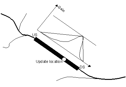
Figure: Definition of gain function for a measurement (update) location.Note that updates cannot take place across river junctions.

The definition of the gain function is illustrated in the definition of gain function for a measurement (update) location.Note that updates cannot. Theoretically, the amplitude reflects the confidence in the observation as compared to the model forecast. That is, if the amplitude equals one, the measurement is as-sumed to be perfect, whereas for smaller amplitudes, less emphasis is put on the measurement as compared to the model forecast. In practice, the amplitude works as an exponential smoothing, because even for low frac-tions the simulation will eventually approach the measurement, due to the correction taking place every simulation time step. An amplitude of one will often result in an instability during the first time steps with updating, due to all of the error being corrected at once during the very first updating step.

With the stationary gain method, an observation only exerts correction of states of the same kind as itself (e.g. if water levels are measured the water level grid points are updated) using the sequential algorithm in Eq. the sequential measurement update for data assimilation processing independent. The principle is that the not-updated states will only receive an indirect update, which is the result of advancing the updated states to the next time step.

The statement about only correcting states of the same kind as the meas-urement comes with a twist:

• A water level measurement corrects water level grid points inside the up-date range, not the discharge grid points.
• A discharge measurement corrects discharge, but the correction is made indirectly, in that the calculated discharge correction is injected as lateral flows to the water level grid points inside the update range - so a dis-charge measurement does not directly manipulate the values of dis-charge grid points.

Error forecast modelling

The filtering procedure described above can be applied to update the state of the river system up to the time of forecast (or as long as measurements are available). This updated state can then be used as initial conditions for a model forecast. In this case, however, the forecast skills of the model will be limited to a time horizon where the initial conditions are washed out. To keep the model on the "right track" for a longer period the filtering procedure is here combined with error forecasts at the measurement points.

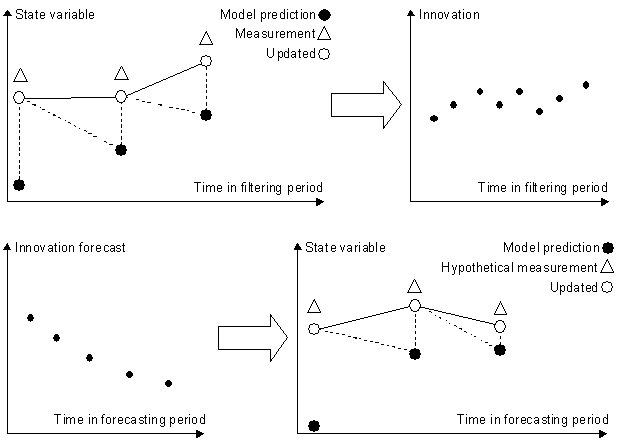
Figure: Illustration of the combined filtering and error forecast procedure.

The principle of this combined approach is illustrated in the illustration of the combined filtering and error forecast procedure. At each update time step in the filtering period (prior to the time of forecast), the model innovation is acquired at all update locations. For each update location this gives rise to a time series of innovations that covers the filtering period up to the time of forecast (or the time of the last measurement). At the end of the filtering period, an error forecast model defined at each update location is then used to propagate the innovation in the forecasting period and update the affected state variables accordingly using the filtering algorithm in Eq. the sequential measurement update for data assimilation processing independent.

The error forecast model can be defined as a general linear or non-linear model with a one-step ahead prediction that depends on the previous innovations (e_k-1, e_k-2, ...), the forecasted model state at the present time step (\(\overline{x}_{k}^{f}\)), the previous updated model states (\(x_{k-1}^a, x_{k-2}^a, \ldots\)), and the present and previous model forcings (u_k, u_k-1, ...)

\[ \varepsilon_k = f(\varepsilon_{k-1}, \varepsilon_{k-2}, \ldots, x_k^f, x_{k-1}^a, x_{k-2}^a, \ldots, u_k, u_{k-1}, \ldots) \]

Equation: Recursive innovation model dependent on prior innovations and forecast model state.

Equation the recursive innovation model dependent on prior innovations and forecast model is used recursively by substituting observed innovations with forecasted values.

In the implementation, an equation parser is used that facilitates an easy and flexible definition of error forecast models such as auto-regressive, moving average models or other linear or non-linear functional forms based on common mathematical operators. Thus, it is possible to define a wide range of error forecast models tailored to the local nature of the model error at each update location.

In order to ensure a fast, accurate and objective derivation of the error forecast models, fully automatic parameter estimation techniques have been incorporated. On the basis of a user-defined time window in the filtering period prior to the time of forecast, the parameters of the error forecast model are estimated. The error forecast models are updated when a new forecast is to be issued using time series of the most recent innovations. This allows the error forecast models to adapt from one forecast to the next to the physical conditions prevailing at the time of forecast without any need for calibration or user intervention in general. In the case of a linear error forecast model, the model parameters are estimated using least squares regression techniques, whereas the shuffled complex evolution (SCE) algorithm (Duan et al. ¹) is applied for the parameter optimisation in the case of a non-linear model.

---

1. Duan, Q., Sorooshian, S., Gupta, V., 1992, Effective and efficient global optimization for conceptual rainfall-runoff models, Water Resour. Res., 28(4), 1015-1031. ↩