Discretisation

Equations the continuity equation relating longitudinal discharge gradient and area changes to and the saint-Venant momentum equation with inertial, pressure gradient, and friction are transformed to a set of implicit finite difference equations on a computational staggered grid consisting of alternating q- and h-grid points, i.e. points where the discharge, q and water level h, respectively, see the reach section with alternating q- and h-grid points.

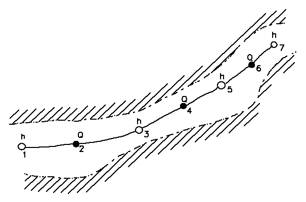
Figure: Computational staggered grid consisting of alternating discharge and water level points.

The computational grid is generated automatically on the basis of the user requirements. q-points are always placed midway between neighbouring h-points, while the distance between h-points may differ. The discharge is defined as positive in the positive x-direction (increasing chainage).

The minimum number of grid points in a reach is three: Two h-grid points and a q-grid point.

The adopted numerical scheme is the implicit 6-point scheme by Abbott and Ionescu (Abbott and Ionescu, 1967), as shown in the reach section with alternating q- and h-grid points. The basic idea is to use values adjacent in time and space to write down the derivative of q and h and thereby convert the two Saint-Venant equations to a set of coupled implicit finite difference equations. Details are given below, first for the continuity equation and then for the momentum conservation equation.

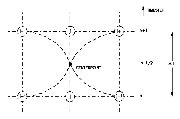
Figure: Abbott scheme for converting Saint-Venant equations to finite difference equations.

To obtain a time centred description, some terms must be available at time level n+½. That can only be fulfilled by iterating. For the first iteration, values at time n+½ are approximated at time n, and in subsequent iterations the values at time n+½ are weighted by values at time n and n+1:

\[ A^{n~+~\delta}~=~\delta A^{n~+~1}+(1-\delta)A^{n} \]

Equation: Time-weighted interpolation of flow area for semi-implicit finite difference scheme.

To get 2nd order accurate approximations \(\delta\)=½ must be used.

The more iterations will provide the best possible time centred values,. The number of iterations can be controlled by the user.

Urban (MIKE+)

MIKE+ does not iterate, and hence always uses the value at time n for the time centred terms.

Continuity equation

The continuity equation is approximated at all h-grid points.

In the continuity equation the storage width, b_s, is introduced as:

\[ \frac{\partial A}{\partial t}~=~b_{s}\frac{\partial h}{\partial t} \]

Equation: Area change expressed through storage width and water level gradient.

giving:

\[ \frac{\partial q}{\partial x} + b_s \frac{\partial h}{\partial t} = q_{in} \]

Equation: Continuity equation in terms of discharge and water level with slot storage.

As only q has a derivative with respect to x, the equation can easily be centred at an h-point, see the centered discretization of the continuity equation.

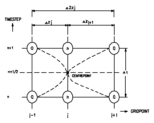
Figure: Centered discretization of the continuity equation.

The approximation of terms Equation the continuity equation in terms of discharge and water level with slot storage are expressed as follows:

\[ \frac{\partial q}{\partial x} \approx \delta \frac{q_{j+1}^{n+1} - q_{j-1}^{n+1}}{\Delta 2 x_j} + (1 - \delta) \frac{q_{j+1}^n - q_{j-1}^n}{\Delta 2 x_j} \]

Equation: Finite difference approximation of spatial discharge gradient using weighted combination of upstream and downstream points.

\[ \frac{\partial h}{\partial t}\!\approx\!\frac{(h_{j}^{n~+~1}-h_{j}^{n})}{\Delta t} \]

Equation: Finite difference approximation of the water level time derivative.

b_s in Equation the continuity equation in terms of discharge and water level with slot storage is retrieved from the cross section at the h grid point.

Urban (MIKE+)

In MIKE+ type setups, b_s in Equation the continuity equation in terms of discharge and water level with slot storage is approximated differently, by:

\[ b_s = \frac{A_{sj-1/2} + A_{sj+1/2}}{\Delta 2x_j} \]

Equation: Surface width approximation from averaged surface areas between grid points.

where:

A_s,j-½   is the surface area between grid point j-1 and j

A_s,j+½   is the surface area between grid point j and j+1

The user can control if this approximation should be used. It will only be applied if the surrounding q-grid-point has a cross section (the MIKE+ fully dynamic scheme has this).

See Section A.3.1 for details on improvement on the mass balance.

Substituting for the derivatives in equation the continuity equation in terms of discharge and water level with slot storage gives a formulation of the following form for h-grid point j:

\[ \alpha_j Q_{j-1}^{n+1} + \beta_j h_j^{n+1} + \gamma_j Q_{j+1}^{n+1} = \delta_j \]

Equation: Discretized continuity equation at h-grid point j in finite difference form.

where, a, b and g are functions of \(b_{s}\) and d and, moreover, depend on q and h at time level n and q on time level n+½.

The continuity equation for h-grid point j in the form the discretized continuity equation at h-grid point j in finite difference form will be used to set up a system of equation in sections A.2.2.

Momentum equation

The momentum equation is centred at q-grid points as illustrated in the centring of momentum equation in the 6-point Abbott scheme.

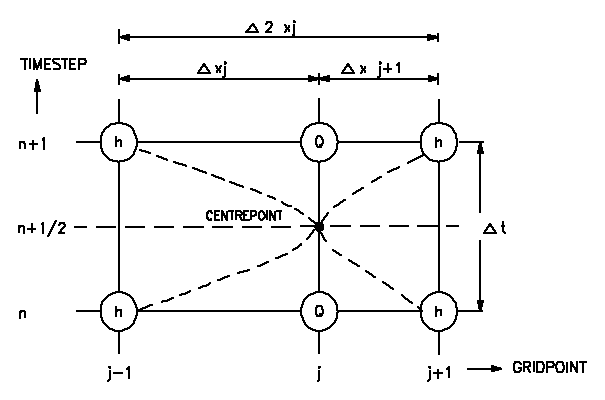
Figure: Centered discretization of the momentum equation.

The approximation of each term in the Momentum Equation the saint-Venant momentum equation with inertial, pressure gradient, and friction differ for each of the schemes. The general approximations will be described first, followed by the special versions for each scheme.

The temporal term is approximated by:

\[ \frac{\partial q}{\partial t} \approx \frac{q_j^{n+1} - q_j^n}{\Delta t} \]

Equation: Finite difference discretization of the discharge time derivative.

The gravity term is approximated by

\[ \frac{\partial h}{\partial x} \approx \delta \frac{h_{j+1}^{n+1} - h_{j-1}^{n+1}}{\Delta 2x_j} + (1 - \delta) \frac{h_{j+1}^n - h_{j-1}^n}{\Delta 2x_j} \]

Equation: Finite difference approximation of water level gradient with weighted temporal interpolation.

With all the terms having their approximation inserted, the momentum equation can be written in the following form:

\[ \alpha_j h_{j-1}^{n+1} + \beta_j q_j^{n+1} + \gamma_j h_{j+1}^{n+1} = \delta_j \]

Equation: Discretised implicit finite-difference form of the momentum equation at a q-grid point.

The conservation of momentum equation for q-grid point j in the form the discretised implicit finite-difference form of the momentum equation at a q-grid will be used to set up a system of equation.

Fully dynamic, higher order, MIKE 11

The momentum term is approximated at time n+½, when available, though in first iteration at time n.

\[ \frac{\partial}{\partial x} \left( a \frac{q^2}{A_{rr}} \right) \approx \frac{\left[ a \frac{q^2}{A_{rr}} \right]_{j+1}^{n+1/2} - \left[ a \frac{q^2}{A_{rr}} \right]_{j-1}^{n+1/2}}{\Delta 2x_j} \]

Equation: Spatial discretization of momentum term at half-time step using velocities and cross-sectional properties.

The friction term is approximated using the higher order approximation of Verwer, described in Section A.2.1.3.

Diffusive wave, MIKE 11

In the diffusive wave approximation, all momentum terms are ignored and only the gravitation and friction terms are maintained. The Momentum Equation reduces to:

\[ Q|Q|~=~-A^{2}C^{R}R\frac{\partial h}{\partial x}=-K^{2}\frac{\partial h}{\partial x} \]

Equation: Diffusive wave approximation relating discharge to water surface slope through conveyance.

where K is conveyance. Using the finite difference approximation of water level gradient with weighted temporal and

\[ Q|Q|\approx Q^{n~+~1}\big|Q^{n}\big| \]

Equation: Time-weighted approximation of the quadratic friction term for diffusive wave routing.

gives

\[ \frac{K^2}{2 \Delta 2x_j |Q^n|} (h_{j+1}^{n+1} - h_{j-1}^{n+1}) + Q^{n+1} + \frac{1}{2} Q^n = 0 \]

Equation: Discretized diffusive wave equation for kinematic wave approximation.

which is of the form the discretised implicit finite-difference form of the momentum equation at a q-grid.

Kinematic wave, MIKE 11

In the kinematic wave approximation, the gravitational term is exactly cancelled by the friction term:

$g A\frac{\partial h}{\partial x}+g A f Q|Q| $

From this simple equation Q is found as a function of h, and the discharge is computed from a Taylor expansion:

\(q_{j}^{n~+~1}=~q_{j}^{n}+\frac{\Delta Q}{\Delta h}(h_{j~+~1}^{n~+~1}-h_{j~+~1}^{n})\)

Fully dynamic, MIKE 11

The momentum term is included partly implicit. To ensure the correct sign for the term when the flow direction is changing during a time step, the semi implicit term is weighted with the explicit term:

\[ q^2 \approx \theta q_j^{n+1} q_j^n - (\theta - 1) q_j^n q_j^n \]

Equation: Semi-implicit weighting of the nonlinear momentum term ensuring correct flow direction.

where q can be specified by the user. The default value of q is 1.0.

Fully dynamic, MIKE+

The momentum term is approximated based on the transformation introduced by Abbott and Ionescu (¹):

\[ \frac{\partial \left(\frac{q^{2}}{A}\right)}{\partial x} = \frac{\partial \left(q \cdot qA^{-1}\right)}{\partial x} = qA^{-1}\frac{\partial q}{\partial x} + Q\frac{\partial \left(qA^{-1}\right)}{\partial x} \]

Equation: Momentum term after the Abbott-Ionescu transformation.

Using the Continuity Equationthe continuity equation in terms of discharge and water level with slot storage to eliminate the q derivative gives:

\[ \frac{\partial \left(\frac{q^{2}}{A}\right)}{\partial x} = qA^{-1}\left(-b_{s}\frac{\partial h}{\partial t} + q_{in}\right) + Q\frac{\partial \left(qA^{-1}\right)}{\partial x} \]

Equation: Momentum term with the discharge derivative eliminated using the continuity equation.

The last term is approximated at time \(n + \delta\), when available, though in first iteration at time n:

\[ Q\frac{\partial \left(qA^{-1}\right)}{\partial x} \approx \left( (1-\delta) q^{n} + \delta q^{n+\delta} \right) \cdot \left( \frac{\left(\frac{q}{A}\right)_{j+1}^{n+\delta} - \left(\frac{q}{A}\right)_{j-1}^{n+\delta}}{\Delta x} \right) \]

Equation: Discretised approximation of the convective acceleration term.

The resistance term in the fully dynamic MIKE+ scheme has several approximations, depending on the resistance formulation. If the resistance formulation is Manning M, in MIKE+ terms called explicit Manning, the term is included in the form:

\[ I_{f} = \frac{\sqrt{I_{h}}}{MAR^{2/3}} \]

Equation: Friction slope term for the explicit Manning resistance formulation.

The user can also specify to use an implicit Manning formulation, in which case the friction term is approximated using the higher order approximation of Verwer, described in Section A.2.1.3.

The 1D engine currently only supports the explicit Manning formulation.

Urban (MIKE+)

In MIKE+, the choice between explicit and implicit flow resistance description is made through the DHIAPP.INI file, see Appendix D.3. The explicit description is selected per default.

Implicit resistance implementation

The resistance term can be approximated using the higher order accurate approximation of Verwer, ². This higher order accurate approximation can greatly improve the stability of the scheme. It is based on a resistance formulation on the form

\[ I_{f} = F = fq\left|q\right| \]

Equation: Friction slope expressed as the momentum forcing term.

where f is a generalised friction factor. The resistance term is approximated at time step n+\(\delta\), i.e. time \(t^{n} + \delta \cdot \Delta t\), using a Taylor expansion around time \(f^{n}\), remembering that the friction factor \(f = f\left(h\right)\) depends on the water level h:

\[ F(t^{n} + \delta \Delta t) = F(t^{n}) + \delta \Delta t\frac{\partial F}{\partial t} = F(t^{n}) + \delta \Delta t\left(\frac{\partial F}{\partial q} \cdot \frac{\partial q}{\partial t} + \frac{\partial F}{\partial h} \cdot \frac{\partial h}{\partial t}\right) \]

Equation: Taylor expansion of the friction term in time.

In terms of values at the time step n, it becomes

\[ F^{n+\delta} \approx F^{n} + \delta\left(\left.\frac{\partial F}{\partial q}\right|^{n} \cdot \Delta q + \left.\frac{\partial F}{\partial h}\right|^{n} \cdot \Delta h\right) \]

Equation: Taylor expansion of friction term for semi-implicit time stepping.

Expanding this gives

\[ F^{n+\delta} \approx f^{n}\left|q^{n}\right|q^{n} + \delta\left(2f^{n}\left|q^{n}\right| \cdot (q^{n+\delta} - q^{n}) + \left|q^{n}\right|q^{n}\left.\frac{\partial f}{\partial h}\right|^{n} \cdot \Delta h\right) \]

Equation: Taylor-expanded approximation of friction term with velocity and water level dependencies.

The friction factor derivative depends on the resistance formulation. For Manning M and Chezy, the factor is based on the conveyance,

\[ K = K(h) = M A R^{2/3} \quad \text{or} \quad C A R^{1/2} \]

Equation: Conveyance formula relating flow capacity to Manning M or Chezy C resistance coefficient, flow area, and hydraulic radius.

where

\[ f = \frac{1}{K^2} = M^{-2} A^{-2} R^{(-4)/3} \quad \text{or} \quad C^{-2}A^{-2}R^{-1} \]

Equation: Friction factor as a function of Manning or Chezy coefficients and hydraulic radius.

This gives the friction factor derivatives:

\[ \frac{\partial f}{\partial h} = -2M^{-3}\frac{\partial M}{\partial h}A^{-2}R^{-4/3} - 2M^{-2}A^{-3}\frac{\partial A}{\partial h}R^{-4/3} - \frac{4}{3}M^{-2}A^{-2}R^{-1}\frac{\partial R}{\partial h} \]

Equation: Derivative of the friction factor with respect to water level, Manning M formulation.

\[ \frac{\partial f}{\partial h} = -2C^{-3}\frac{\partial C}{\partial h}A^{-2}R^{-1} - 2C^{-2}A^{-3}\frac{\partial A}{\partial h}R^{-1} - C^{-2}A^{-2}R^{-2}\frac{\partial R}{\partial h} \]

Equation: Derivative of the friction factor with respect to water level, Chezy C formulation.

which can be simplified to

\[ \frac{\partial f}{\partial h} = f\left(-2M^{-1}\frac{\partial M}{\partial h} - 2A^{-1}\frac{\partial A}{\partial h} - \frac{4}{3}R^{-1}\frac{\partial R}{\partial h}\right) \]

Equation: Simplified derivative of the friction factor, Manning M formulation.

\[ \frac{\partial f}{\partial h} = f\left(-2C^{-1}\frac{\partial C}{\partial h} - 2A^{-1}\frac{\partial A}{\partial h} - R^{-1}\frac{\partial R}{\partial h}\right) \]

Equation: Simplified derivative of the friction factor, Chezy C formulation.

The \(\Delta h\) term is approximated at the h grid point in the flow upstream direction, i.e.

\[ \Delta h = h_{us}^{n+1} - h_{us}^{n-1} \]

Equation: Water level increment used for the time-centred friction term.

where

\[ h_{u s}=\left\{\begin{array}{l l}{h_{j-~1}~~\mathrm{if}~~(q_{j}>0)}\\ {h_{j+~1}~~\mathrm{if}~~(q_{j}<0)}\end{array}\right. \quad \text{and} \quad h_{d s}=\left\{\begin{array}{l l}{h_{j~+~1}~~\mathrm{if}~~(q_{j}>0)}\\ {h_{j~-~1}~~\mathrm{if}~~(q_{j}<0)}\end{array}\right. \]

Equation: Selection of upstream and downstream water levels based on flow direction for friction calculation.

The coefficient d determines the time weighting of the scheme. For stability reasons the coefficient should be above 0.5.

---

1. Abbott, M.B. and Ionescu, F.: On the numerical computation of nearly-horizontal flows. J.Hyd.Res., 5, 1967, pp. 97-117. ↩

2. Verwey, A.: Linkage of Physical and Numerical Aspects of Models Applied in Environmental Studies. Keynote lecture. In: Proceedings of the Conference on Hydraulics in Civil Engineering. International Conference on Hydraulics in Civil Engineering, 15–17 February 1994, Brisbane, Australia. ↩