Conservation of momentum

Conservation of momentum

\[ \frac{\partial(\rho H b\bar{u})}{\partial t} = -\frac{\partial\left(\alpha' \rho H b \bar{u}^2 + \frac{1}{2}\rho g b H^2\right)}{\partial x} \]

Equation: Momentum balance in a channel accounting for inertial, convection, and pressure forces.

where r is the density, H the depth, b the width, \(\bar{u}\) the average velocity along the vertical and a’ the vertical velocity distribution coefficient.

Introducing the bottom slope, I_b, and allowing for the channel width to vary will give rise to two more terms in the momentum equation. These terms describe the projections in the flow direction of the reactions of the bottom and side walls to the hydrostatic pressure.

The momentum equation now becomes:

\[ \frac{\partial \left(\rho H b \overline{u}\right)}{\partial t} = -\frac{\partial \left(\alpha' \rho H b \overline{u}^{2} + \frac{1}{2}\rho g b H^{2}\right)}{\partial x} + \frac{\partial b}{\partial x}\frac{\rho g H^{2}}{2} - \rho g H b I_{b} = -\frac{\partial \left(\alpha' \rho H b \overline{u}^{2}\right)}{\partial x} - b\frac{\partial \left(\frac{1}{2}\rho g H^{2}\right)}{\partial x} - \rho g H b I_{b} \]

Equation: The momentum equation with the bottom slope and varying channel width terms included.

When the water level, h, is introduced into the relationship instead of water depth:

\[ \frac{\partial h}{\partial x}=~I_{b}+\frac{\partial H}{\partial x} \]

Equation: Water level gradient expressed as a function of bottom slope and channel width variation.

and the equations are divided by r, the conservation laws of mass and momentum become:

\[ \frac{\partial \left(\rho Hb\right)}{\partial t} = -\frac{\partial \left(\rho Hb\overline{u}\right)}{\partial x} \]

Equation: Conservation of mass for water density, cross-section height, and discharge per unit width.

\[ \frac{\partial(Hb\bar{u})}{\partial t} = -\frac{\partial(\alpha' Hb\bar{u}^2)}{\partial x} - Hbg\frac{\partial h}{\partial x} \]

Equation: Conservation of momentum for a shallow water flow accounting for density, depth, velocity, and pressure gradient.

These equations can be integrated to describe the flow through cross sections of any shape when divided up into a series of rectangular cross sections as shown in the cross section divided into a series of rectangular channels:

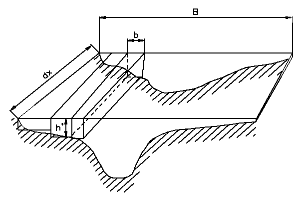
Figure: Cross section divided into a series of rectangular channels.

According to the previous assumptions, \(\frac{\partial h}{\partial x}\) is constant across the channel and no exchange of momentum occurs between the sub-channels. If the integrated cross section area is called A and the integrated discharge q, and B is the full width of the channel, then:

\[ A = \int_0^B H \, db \]

Equation: Integrated cross-sectional flow area across the channel width.

\[ q=\int_{0}^{B}H\overline{u}{\mathrm{d}}b~=~\overline{u}A \]

Equation: Discharge as the product of mean flow velocity and integrated cross-sectional area.

Integrating the mass and momentum conservation equations and introducing Equations the integrated cross-sectional flow area across the channel width and the discharge as the product of mean flow velocity and integrated cross-sectional yields:

\[ \frac{\partial q}{\partial x}+\frac{\partial A}{\partial t}\quad0 \]

Equation: Continuity equation relating discharge and area changes along the reach.

\[ \frac{\partial q}{\partial t}+\frac{\partial\!\left(\alpha\frac{q^{2}}{A}\right)}{\widehat{\sigma}x}+g A\frac{\partial h}{\widehat{\sigma}x}=~0 \]

Equation: Shallow-water momentum equation integrating acceleration, momentum flux, and water surface slope.

Including the flow resistance term in the form as a friction slope, a lateral inflow \(q_{in}\),and an external momentum forcing f into these equations leads to the basic equations used in the 1D engine:

\[ \frac{\partial Q}{\partial x}+\frac{\partial A}{\partial t}~=~q_{i n} \]

Equation: Continuity equation relating longitudinal discharge gradient and area changes to lateral inflow.

\[ \frac{\partial q}{\partial t} + \frac{\partial\left(\alpha \frac{q^2}{A}\right)}{\partial x} + gA\frac{\partial h}{\partial x} + gAI_f = f \]

Equation: Saint-Venant momentum equation with inertial, pressure gradient, and friction terms.

Pressurised Flow, Generalisation of Saint-Venant Equations

The idea of introducing a fictitious slot was first presented by Preissmann and Cunge, 1961 /2/, and has since been used by Cunge and Wegner, 1964 /1/.

To show that a top slot can be included without modifying the Saint-Venant equations, we start by rewriting the continuity equation as:

\[ -\frac{\partial(\rho Q)}{\partial x} dx dt = \frac{\partial(\rho A)}{\partial t} dx dt \]

Equation: Continuity equation relating the spatial change in mass flux to the temporal change in cross-sectional area.

assuming the density of water r is constant over the cross section.

By partial differentiation we find:

\[ \frac{\partial Q}{\partial x} + \frac{Q}{\rho}\frac{\partial \rho}{\partial x} + \frac{\partial A}{\partial t} + \frac{A}{\rho}\frac{\partial \rho}{\partial t} = 0 \]

Equation: Continuity equation accounting for variable density in a compressible water column.

For a circular closed reach, it can be shown that the density of the water can be approximated as:

\[ \rho\approx\!\rho_{0}\!\left(1+\frac{g(y-D)}{{{a}_{0}}^{2}}\right) \]

Equation: Density of water in a pressurized closed pipe accounting for compressibility.

where:

• r_o — the density of water for a free surface flow [kgm^-3]
• a_o — the speed of sound in water [ms^-1]
• y — the water depth [m]
• D — the reach diameter [m]. Furthermore, it can be shown that the cross section area in the case of the excess pressure rg(y-D) is approximately equal to:

\[ A\approx A_{0}\bigg(1+\frac{g(y-D)}{{a_{r}}^{2}}\bigg) \]

Equation: Cross-sectional area expansion due to excess pressure in a pressurized reach.

where

A_o = the area without excess pressure and a_r is given as:

\[ {a}_{r}~=~\sqrt{\frac{{E}_{r}\cdot{e}}{{\rho}_{0}\cdot{D}}} \]

Equation: Acoustic wave speed in water accounting for Young's modulus and pipe elasticity.

and

E_r = the Young`s modulus of elasticity, [Nm^-2] e = the reach wall thickness, [m].

The a_r has the dimension ms^-1 and is in the order of 1400 ms^-1 for most concrete pipes.

Combining these equations yields:

\[ \frac{\partial A}{\partial t} + \frac{A}{\rho} \cdot \frac{\partial \rho}{\partial t} = g \cdot A\frac{\partial y}{\partial t}\left(\frac{1}{a_r^2} + \frac{1}{a_0^2}\right) = \frac{gA_0}{a^2} \cdot \frac{\partial y}{\partial t} \]

Equation: Relation between cross-sectional area, density, and water level changes in pressurised pipe flow.

where:

\[ a~=~\frac{a_{0}}{\sqrt{1a_{0}^{2}/a_{r}^{2}}} \]

Equation: Speed of sound in water accounting for fluid compressibility and pipe wall elasticity.

represents the speed of sound in water considering the compressibility of water and the deformation of the reach wall.

Equation the continuity equation accounting for variable density in a compressible water can now be written as:

\[ \frac{\partial Q}{\partial x} + \frac{Q}{\rho} \cdot \frac{\partial \rho}{\partial x} + \frac{gA_0}{a^2} \cdot \frac{\partial y}{\partial t} = 0 \]

Equation: Compressible flow continuity equation accounting for density gradients and water elasticity through speed of sound.

If we further assume that the density of water varies only slowly along the reach so that

\[ \frac{\partial \rho}{\partial x} = 0 \]

Equation: Assumption that water density remains constant along the longitudinal direction.

and use that the cross section area for water level in the slot varies as:

\[ \frac{\partial A}{\partial t} = b_{slot} \frac{\partial y}{\partial t} \]

Equation: Rate of change of cross-sectional area with water level in a flow slot.

then the continuity equation can be recovered by choosing the slot width so that

\[ b_{s l o t}=\frac{g A_{0}}{a^{2}} \]

Equation: Slot width for fictitious slot method ensuring continuity equation recovery.

a is in the order of 1000 [ms^-1] for most concrete pipes.

Solving the Saint-Venant Equations

This chapter describes how the Saint-Venant equations are solved. First, the equations are discretised on a grid in Section A.2.1, then the method of solving the resulting equations is presented in sections A.2.2. In the last two sections it is described how boundaries (Section A.2.3) and structures (Section A.2.4) are included.

Discretisation

Equations the continuity equation relating longitudinal discharge gradient and area changes to and the saint-Venant momentum equation with inertial, pressure gradient, and friction are transformed to a set of implicit finite difference equations on a computational staggered grid consisting of alternating q- and h-grid points, i.e. points where the discharge, q and water level h, respectively, see the reach section with alternating q- and h-grid points.

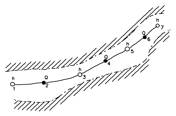
Figure: Reach section with alternating q- and h-grid points.

The computational grid is generated automatically on the basis of the user requirements. q-points are always placed midway between neighbouring h-points, while the distance between h-points may differ. The discharge is defined as positive in the positive x-direction (increasing chainage).

The minimum number of grid points in a reach is three: Two h-grid points and a q-grid point.

The adopted numerical scheme is the implicit 6-point scheme by Abbott and Ionescu (Abbott and Ionescu, 1967), as shown in the reach section with alternating q- and h-grid points. The basic idea is to use values adjacent in time and space to write down the derivative of q and h and thereby convert the two Saint-Venant equations to a set of coupled implicit finite difference equations. Details are given below, first for the continuity equation and then for the momentum conservation equation.

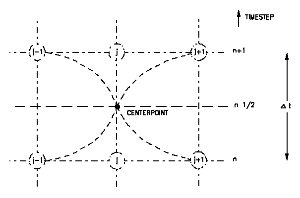
Figure: Centred 6-point Abbott scheme.

To obtain a time centred description, some terms must be available at time level n+½. That can only be fulfilled by iterating. For the first iteration, values at time n+½ are approximated at time n, and in subsequent iterations the values at time n+½ are weighted by values at time n and n+1:

\[ A^{n~+~\delta}~=~\delta A^{n~+~1}+(1-\delta)A^{n} \]

Equation: Time-weighted interpolation of flow area for semi-implicit finite difference scheme.

To get 2nd order accurate approximations \(\delta\)=½ must be used.

The more iterations will provide the best possible time centred values,. The number of iterations can be controlled by the user.

Urban (MIKE+)

MIKE+ does not iterate, and hence always uses the value at time n for the time centred terms.

Continuity equation

The continuity equation is approximated at all h-grid points.

In the continuity equation the storage width, b_s, is introduced as:

\[ \frac{\partial A}{\partial t}~=~b_{s}\frac{\partial h}{\partial t} \]

Equation: Area change expressed through storage width and water level gradient.

giving:

\[ \frac{\partial q}{\partial x} + b_s \frac{\partial h}{\partial t} = q_{in} \]

Equation: Continuity equation in terms of discharge and water level with slot storage.

As only q has a derivative with respect to x, the equation can easily be centred at an h-point, see the centring of the continuity equation in the 6-point Abbott scheme.

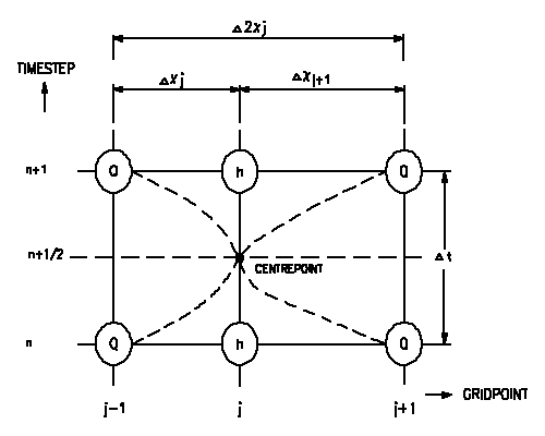
Figure: Centring of continuity equation in 6-point Abbott scheme.

The approximation of terms Equation the continuity equation in terms of discharge and water level with slot storage are expressed as follows:

\[ \frac{\partial q}{\partial x} \approx \delta \frac{q_{j+1}^{n+1} - q_{j-1}^{n+1}}{\Delta 2 x_j} + (1 - \delta) \frac{q_{j+1}^n - q_{j-1}^n}{\Delta 2 x_j} \]

Equation: Finite difference approximation of spatial discharge gradient using weighted combination of upstream and downstream points.

\[ \frac{\partial h}{\partial t}\!\approx\!\frac{(h_{j}^{n~+~1}-h_{j}^{n})}{\Delta t} \]

Equation: Finite difference approximation of the water level time derivative.

b_s in Equation the continuity equation in terms of discharge and water level with slot storage is retrieved from the cross section at the h grid point.

Urban (MIKE+)

In MIKE+ type setups, b_s in Equation the continuity equation in terms of discharge and water level with slot storage is approximated differently, by:

\[ b_s = \frac{A_{sj-1/2} + A_{sj+1/2}}{\Delta 2x_j} \]

Equation: Surface width approximation from averaged surface areas between grid points.

where:

A_s,j-½ is the surface area between grid point j-1 and j

A_s,j+½ is the surface area between grid point j and j+1

The user can control if this approximation should be used. It will only be applied if the surrounding q-grid-point has a cross section (the MIKE+ fully dynamic scheme has this).

See Section A.3.1 for details on improvement on the mass balance.

Substituting for the derivatives in equation the continuity equation in terms of discharge and water level with slot storage gives a formulation of the following form for h-grid point j:

\[ \alpha_j Q_{j-1}^{n+1} + \beta_j h_j^{n+1} + \gamma_j Q_{j+1}^{n+1} = \delta_j \]

Equation: Discretized continuity equation at h-grid point j in finite difference form.

where, a, b and g are functions of \(b_{s}\) and d and, moreover, depend on q and h at time level n and q on time level n+½.

The continuity equation for h-grid point j in the form the discretized continuity equation at h-grid point j in finite difference form will be used to set up a system of equation in sections A.2.2.

Momentum equation

The momentum equation is centred at q-grid points as illustrated in the centring of momentum equation in the 6-point Abbott scheme.

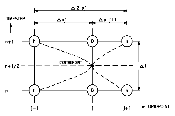
Figure: Centring of momentum equation in the 6-point Abbott scheme.

The approximation of each term in the Momentum Equation the saint-Venant momentum equation with inertial, pressure gradient, and friction differ for each of the schemes. The general approximations will be described first, followed by the special versions for each scheme.

The temporal term is approximated by:

\[ \frac{\partial q}{\partial t} \approx \frac{q_j^{n+1} - q_j^n}{\Delta t} \]

Equation: Finite difference discretization of the discharge time derivative.

The gravity term is approximated by

\[ \frac{\partial h}{\partial x} \approx \delta \frac{h_{j+1}^{n+1} - h_{j-1}^{n+1}}{\Delta 2x_j} + (1 - \delta) \frac{h_{j+1}^n - h_{j-1}^n}{\Delta 2x_j} \]

Equation: Finite difference approximation of water level gradient with weighted temporal interpolation.

With all the terms having their approximation inserted, the momentum equation can be written in the following form:

\[ \alpha_j h_{j-1}^{n+1} + \beta_j q_j^{n+1} + \gamma_j h_{j+1}^{n+1} = \delta_j \]

Equation: Discretised implicit finite-difference form of the momentum equation at a q-grid point.

The conservation of momentum equation for q-grid point j in the form the discretised implicit finite-difference form of the momentum equation at a q-grid will be used to set up a system of equation.