Bridges

MIKE 1D offers a number of approaches when modelling flow through bridges. The approach to choose should be based on the assumptions for the different methods and the requirements for the modelling.

The bridge modelling approaches can be divided into pure free flow methods and methods which may be combined with submergence/overflow methods. The pure free flow methods can be further sub-divided into methods for piers and methods for arches.

The methods specially designed for piers are

• Bridge Piers (Nagler) (p. 142): An orifice type of flow description with the effect of the piers taken into account through an adjustment factor.
• Bridge Piers (Yarnell) (p. 143): An equation derived from experiments for normal flow conditions in the sub critical flow range. Again the effect of piers is handled through the use of adjustment factors.

The free flow arch methods available are

• Arch Bridges (Biery and Delleur) (p. 139): An orifice type of equation is used to describe the discharge through the bridge. The equation is derived under the assumption of a rectangular channel and is based on a single span arch opening. Multiple arch openings are handled by a simple multiplication factor.
• Arch Bridges (Hydraulics Research (HR) method) (p. 140): The HR method is based on laboratory experiments of both single and multi spanned arch bridges in rectangular channels. The method uses tables describing the relation between the blockage ratio, the downstream Froude number and the upstream water level.

The methods than can be combined with both submergence and overflow methods are the following

• Energy Equation (p. 144): A standard step method where a backwater surface profile is determination is used to calculate the discharge through the bridge. The method takes the contraction and expansion loss for bridges of arbitrary shape into account. The method assumes sub-critical flow and may default to critical flow for steep water surface gradients.
• Federal Highway Administration (FHWA) WSPRO method (p. 147): The FHWA WSPRO method is based on the solution of the energy equation. Contraction loss is taken into account through the calculation of an effective flow length. Expansion losses are determined through the use of numerous experimentally based tables. The method takes the effect of eccentricity, skewness, wingwalls, embankment slope etc. into account through the use of these tables.
• US Bureau of Public Roads (USBPR) method (p. 157): The USBPR method estimates free-surface flow assuming normal depth conditions. the method is based on experiments and takes the effect of eccentricity, skewness and piers into account.

The submergence methods available are

• Pressure Flow, Federal Highway Administration method (p. 159): Two orifice equation descriptions are used. One for situations when the orifice is submerged downstream and modified equation for situations when only the upstream part of the orifice is submerged.
• MIKE 1D culvert: A standard MIKE 1D culvert description may be chosen for submergence flow. The culvert to be used is specified by the user. The culvert is only active if submergence occurs.
• Energy equation: The flow under the bridge is determined through a standard backwater step method. The flow is assumed to be in the sub-critical range and thus the method may default to critical flow. Both contraction and expansion loss is taken into account.

Overflow methods available are:

• Energy Equation: The flow over the bridge is determined through a standard backwater step method. The flow is assumed to be in the sub-critical range and thus the method may default to critical flow. Both contraction and expansion loss is taken into account.
• Road overflow, Federal Highway Administration method (p. 162): The overflow is modelled using a weir equation taking tail water submergence into account through the use of a submergence coefficient. The method may be used for both gravel and paved surfaces.
• MIKE 1D weir: A standard MIKE 1D weir description may be chosen for overflow. The weir to be used is specified by the user. The weir is only active if overflow occurs.

Arch Bridges (Biery and Delleur)

The Biery and Delleur method is specially designed for semi circular arch bridges. It does not consider skewness, eccentricity, entrance rounding or piers (²). The method is based on experiments carried out for a rectangular channel.

The discharge, Q, through a semicircular arch in a rectangular channel is calculated from:

\[ Q = 0.7083 C_{D}(2g)^{1/2}Y_{us}^{3/2}b\left[1 - 0.1294\left(\frac{Y_{us\text{-}Lim}}{r}\right)^{2} - 0.0177\left(\frac{Y_{us\text{-}Lim}}{r}\right)^{4}\right] \]

Equation: Discharge through a fully submerged arch bridge, Hydraulics Research (HR) method.

where

\(C_{D}\)  Coefficient of discharge.

\(g\)  Acceleration due to gravity.

\(Y_{us}\)  Average water depth upstream of the bridge (= Area_us/Width_us).

\(b\)  Opening width of the arch.

\(r\)  Radius of curvature.

Given that the discharge will decrease for high values of \(Y_{us}\) a limit corresponding to the maximum discharge is set for \(Y_{us\text{-}Lim}\) :

\[ Y_{us\text{-}Lim} = \begin{cases} Y_{us} & \text{for } \dfrac{Y_{us}}{r} < 1.49555 \\[1.5ex] 1.49555 r & \text{for } \dfrac{Y_{us}}{r} \geq 1.49555 \end{cases} \]

Equation: Limited upstream depth used in the HR method discharge formula, capped once the depth-to-radius ratio exceeds 1.49555.

The upstream depth  \(Y_{us}\) is taken as the average depth in the upstream cross section. Upstream direction is based on the water level gradient. The coefficient of discharge \(C_{D}\) varies with the bridge opening ratio M and the downstream Froude number \(F_{ds}\) . The default table in MIKE 1D is for a semicircular arch models (/5/).

The downstream Froude number \(F_{ds}\) is given by:

\[ F_{ds} = \frac{Q}{A_{ds}}\sqrt{\frac{\alpha_{ds}}{gY_{ds}}} \]

Equation: Downstream Froude number for the HR method.

Where

\(Q\)    Discharge.

\(A_{ds}\)    Total flow area of downstream cross section.

\(\alpha_{ds}\)   Velocity coefficient in downstream cross section (see eq. the velocity distribution coefficient, from the subsection conveyances at).

\(g\)    Acceleration due to gravity.

\(Y_{ds}\)    Average depth in downstream cross section (= Area_ds/Width_ds).

The bridge opening ratio M is defined as the ratio between \(b\) ~ ~and \(B\) :

\[ 1 -\frac{b}{B} \]

Equation: Bridge blockage ratio as complement of opening width to total channel width.

Where

\(b\)   Opening width of the arch (user defined).

\(B\)   Surface width at upstream cross section.

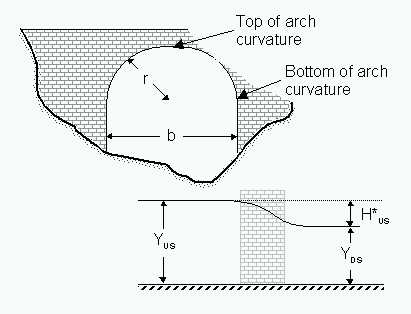
Figure: Hydraulic variables for Biery and Delleur and HR Arch Bridge.

The Biery and Delleur method assumes that the water surface is free i.e. submergence is not taken into account. If the bridge that is being modelled is submerged or over topped an alternative modelling method should be chosen.

Arch Bridges (Hydraulics Research (HR) method)

The Hydraulics Research method estimates the discharge through an arch bridge by the use of a table describing the relation between the upstream afflux, the blockage ratio and the Froude number. The upstream afflux is defined as the increase in water level from normal depth caused by the bridge. The afflux should theoretically be determined one bridge span upstream of the bridge. Thus as a rule of thumb the upstream cross section should be found one bridge span upstream the bridge opening. The default table in MIKE 1D is valid for semicircular arch models (/5/).

\(H_{us}^{\text{*}}\)    The afflux at the upstream cross section of the bridge.

\(Y_{ds}\)   Average depth of flow downstream the bridge (Area_ds/Width_ds).

\(J_{us}\)  The upstream blockage ratio defined as  \(J_{us} = \frac{b_{arch}}{b_{us}}\) .

\(b_{arch}\)   The user defined width of the arch.

\(b_{us}\)    Upstream water surface width.

\(F_{ds}\)    Froude number downstream of the bridge.

The upstream afflux is defined as:

\[ H_{us}^{*} = h_{us} - h_{ds} - \left(\frac{Q}{K_{ds}}\right)^{2}L_{us\text{-}ds} \]

Equation: Upstream afflux, US Federal Highway Administration (FHWA) WSPRO method.

Where:

\(h_{us}\) Water level at upstream cross section.

\(h_{ds}\) Water level at downstream cross section.

\(Q\) Discharge.

\(K_{ds}\) Conveyance in downstream cross section.

\(L_{us\text{-}ds}\) Distance from upstream to downstream cross section.

MIKE 1D determines the discharge based on the upstream and downstream water level. From the afflux and the upstream blockage ratio a Froude number can be determined through the use of the table expressing the relation between afflux and Froude number. For fixed water levels the Froude number depends solely on the discharge. Since the afflux depends on the discharge an iterative process is needed. If the iterative process does not converge the code defaults to critical discharge at the upstream cross section.

The hydraulic research method assumes that the water surface is free i.e. submergence is not taken into account. If the bridge that is being modelled is submerged or over topped an alternative modelling method should be chosen.

Bridge Piers (Nagler)

The Nagler equation is experimentally based. The equation is applicable to bridge piers with different pier shapes. The pier shape is taken into account through a so-called coefficient of discharge which is found through a table based on the pier type. The equation is derived from free flow experiments and is not accurate for high velocities (/7/).

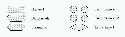
Figure: Type of pier shapes.

The Nagler equation reads:

\[ Q = K_{N}b\sqrt{2g}\left(Y_{ds} - \theta\frac{V_{ds}^{2}}{2g}\right)\left(h_{us} - h_{ds} + \beta\frac{V_{us}^{2}}{2g}\right)^{1/2} \]

Equation: Discharge through the bridge opening, expressed via the downstream depth and velocity heads on both sides.

where:

K_N   Coefficient of discharge.

\(\theta\)    Adjustment factor (default 0.3).

\(\frac{h}{H}\)   Adjustment factor varies with the bridge opening ratio.

g   Acceleration due to gravity.

Y_ds   Depth downstream of the bridge.

V_us   Velocity upstream the bridge.

V_ds   Velocity downstream the bridge.

h_us   Water level in the upstream cross section.

h_ds   Water level in the downstream cross section.

b   The total bridge opening width excluding the piers.

The coefficient of discharge K_N varies with the bridge opening ratio M and the pier shape. The adjustment factor \(\frac{h}{H}\)   varies with the bridge opening ratio M and the adjustment factor \(\theta\)   can normally be taken as 0.3. The default tables in MIKE 1D are after Yarnell and Nagler.

The bridge opening ratio M is defined as the ratio between the flow width in the bridge and the flow width upstream of the bridge b/B.

b   Opening width of the arch.

B   Opening width at upstream cross section.

Eq. the discharge through the bridge opening, expressed via the downstream depth and can be rewritten as a polynomial of third degree in the discharge squared. In case of multiple roots the smallest positive root is chosen as the solution.

The structure area is defined as the arch width times the minimum water depth upstream or downstream.

Bridge Piers (Yarnell)

Like the Nagler equation, the Yarnell equation considers different pier shapes (see the type of pier shapes). The pier shape is accounted for through the so-called pier coefficient. The Yarnell equation is a pure experimentally based equation. The equation assumes free flow. Thus if submergence and possible overtopping is to be modelled an alternative method should be used.

The Yarnell equation reads:

\[ h_{us} - h_{ds} = KY_{ds}F_{ds}^{2}\left(K + 5F_{ds}^{2} - 0.6\right)\left(\alpha + 15\alpha^{4}\right) \]

Equation: Afflux equation relating the upstream/downstream depth difference to the downstream Froude number and blockage ratio.

\[ F_{ds}^{2} = \frac{Q^{2}}{A_{ds}^{2}2gY_{ds}} \]

Equation: Downstream Froude number squared, expressed through discharge, area and depth.

\[ \alpha = 1 - \frac{b}{B_{us}} \]

Equation: Blockage ratio used in the afflux equation.

where

K   Yarnell’s Piers shape Coefficient.

g   Acceleration due to gravity.

Y_ds   Depth downstream the bridge.

F_ds   Froude number downstream the bridge.

\(\alpha\)   Channel contraction ratio.

A_ds   Total flow area of downstream cross section.

b   The bridge opening width excluding the piers.

B_us   The width of the upstream cross section.

h_us   Water level in the upstream cross section.

h_ds   Water level in the downstream cross section.

The default tables for pier shape coefficient K are after Yarnell.

Eq. the afflux equation relating the upstream/downstream depth difference to the may be re-written as a polynomial of second order in the Froude number squared. If multiple positive roots are present the greatest discharge is chosen.

The structure area is defined as the arch width times the minimum water depth upstream or downstream.

Energy Equation

The energy equation may be used to determine the discharge and the back water profile through the bridge. The energy equation takes friction loss and contraction/expansion losses into account. The method requires four cross sections (see the location of cross-sections). River cross sections one and four are defined in the cross-section editor. Bridge cross sections two and three are defined through the bridge geometry in the network editor. Ideally the distance between the bridge and the up- and downstream cross-sections should be of the order b, where b is the bridge opening width. The latter is to ensure that the streamlines are parallel at section one and section four.

The equation solved from section i to i-1 reads

\[ h_{i -1} + h_{v\left(i -1\right)} = h_{i} + h_{vi} + h_{f\left(i, i -1\right)} + h_{e\left(i, i -1\right)} \]

Equation: Energy equation for bridge flow including water level, velocity head, friction, and expansion losses.

where:

h_iWater level at cross-section i.

h_viVelocity head at cross-section i.

h_f(i,i-1)Friction losses between cross-section i and i-1.

h_e(i,i-1)Expansion losses between cross-section i and i-1.

The velocity head is defined as

\[ h_{v} = \frac{\alpha Q^{2}}{2gA^{2}} \]

Equation: Velocity head at a cross section.

with the velocity distribution coefficient defined as

\[ \alpha = \dfrac{\sum\limits_{i=1}^{N}\left(k_{i}^{3}/a_{i}^{2}\right)}{K^{3}/A^{3}} \]

Equation: Velocity distribution coefficient, from the subsection conveyances at cross-section i.

\[ k_{i} = \frac{a_{i}r_{i}^{2/3}}{n_{i}} \]

Equation: Conveyance contribution of a single subsection of a compound cross section.

\[ K = \sum_{i=1}^{N}k_{i} \]

Equation: Total conveyance as the sum of the subsection conveyances.

\[ A = \sum_{i = 1}^{N}a_{i} \]

Equation: Total conveyance as sum of conveyances from individual bridge cross-section subsections.

Where

Q   Discharge at the section.

\(\alpha\)    Velocity distribution coefficient.

k   Subsection conveyance.

a   Subsection area.

K   Total cross section conveyance.

A   Total cross section area.

r   Hydraulic radius.

n   Manning’s roughness coefficient.

NNumber of subsections.

Eq. the velocity distribution coefficient, from the subsection conveyances at is based on a parallel channel analysis. Each parallel channel being defined through subsections. A subsection is understood as segments in series with a constant relative resistance. Further a sub-division may also be achieved through the use of markers 4 and 5. Thus for a cross section with constant relative resistance and no markers 4 or 5 the velocity coefficient is unity. Friction loss. The friction loss between cross-sections i and i-1 is calculated from:

\[ h_{f(i,i-1)} = \frac{L_{i,i-1}Q^{2}}{K_{i}K_{i-1}} \]

Equation: Friction loss between consecutive cross sections i-1 and i.

Where:

L_i,i-1The flow length in the approach reach.

K_iThe conveyance for cross-section i. Expansion/Contraction loss. Expansion/contraction losses are only considered from section 4 to section 3 and from section 2 to section 1. The expansion/contraction loss from section i to section i-1 is expressed as

\[ h_{e(i,i-1)} = C\left|\frac{\alpha_{i}V_{i}^{2}}{2g} - \frac{\alpha_{i-1}V_{i-1}^{2}}{2g}\right| \]

Equation: Expansion/contraction (eddy) loss between consecutive cross sections i-1 and i.

where C is the contraction/expansion coefficient. This coefficient is non-dimensional and is user defined with a value between 0 and 1. the default values are 0.3 for contraction and 0.5 for expansion indicating that the losses due to expansion are typically larger than the losses due to contraction. The solution method. The energy equation method assumes that the flow through the bridge is sub-critical. Further the method is an iterative method. The bridges are pre-calculated based on a set of values for the water levels upstream and downstream. Thus for each set of water level values a discharge is to be determined. The algorithm for determining the discharge has the following steps:

1. Initial guess for the discharge.

2. Backwater calculation from section 4 to section 3.

3. Backwater calculation from section 3 to section 2 based on the result from step 2.

4. Backwater calculation from section 2 to section 1 based on the result from step 3.

5. The water level determined through step 4 is compared with the actual water level at section 1.

6. Based on the comparison in step 5 the discharge is either modified and the algorithm returns to step 2 or the algorithm terminates if the deviation is within acceptable limits.

Throughout the calculation the results are compared with critical flow. If the solution found is below critical water level or if one of the steps 2 - 4 do not converge the code defaults to critical flow at that location. Further if the maximum number of iterations (default 50) is reached without obtaining a valid solution the code defaults to critical flow at section one.

Federal Highway Administration (FHWA) WSPRO method

The computations of the Federal Highway Administration’s WSPRO computer program have been adapted for the calculation of free-surface flow. Some modifications have been necessary in order to fit the MIKE 1D terminology.

The method is based on a standard step method using the energy equation to find the discharge and the backwater water surface profile through the bridge. The method requires four cross sections (see the location of cross-sections). River cross sections one and four are defined in the cross-section editor. Bridge cross sections two and three are defined through the bridge geometry in the network editor. Ideally the distance between the bridge and the up- and downstream cross-sections should be of the order b, where b is the bridge opening width.

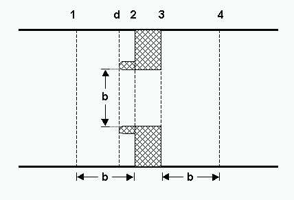
Figure: Location of cross-sections.

The total energy equation between section one and four can be written:

\[ h_{1} + h_{v1} = h_{4} + h_{v4} + h_{f} + h_{e} \]

Equation: Energy balance between the approach section and the bridge exit section, including friction and eddy losses.

where:

h₁Water level at cross-section 1.

h_v1Velocity head at cross-section 1.

h₄Water level at cross-section 4.

h_v4Velocity head at cross-section 4.

h_fFriction losses between cross-section 1 and 4.

h_eExpansion losses between cross-section 3 and 4.

The velocity head is defined as

\[ h_{v} = \frac{\alpha Q^{2}}{2gA^{2}} \]

Equation: Velocity head, restated for the total energy equation between sections 1 and 4.

with the velocity distribution coefficient defined as

\[ \alpha = \dfrac{\sum\limits_{i=1}^{N}\left(k_{i}^{3}/a_{i}^{2}\right)}{K^{3}/A^{3}} \]

Equation: Velocity distribution coefficient, restated for the total energy equation between sections 1 and 4.

\[ k_{i} = \frac{a_{i}r_{i}^{2/3}}{n_{i}} \]

Equation: Conveyance contribution of a single subsection, restated for the total energy equation.

\[ K = \sum_{i=1}^{N}k_{i} \]

Equation: Total conveyance as the sum of the subsection conveyances, restated for the total energy equation.

\[ A = \sum_{i = 1}^{N}a_{i} \]

Equation: Total flow area as sum of subsection flow areas.

Where

Q   Discharge at the section.

\(\alpha\)  Velocity distribution coefficient.

k   Subsection conveyance.

a   Subsection area.

K   Total cross section conveyance.

A   Total cross section area.

r   Hydraulic radius.

n   Manning’s roughness coefficient.

NNumber of subsections.

Eq. the velocity distribution coefficient, from the subsection conveyances at is based on a parallel channel analysis. Each parallel channel being defined through subsections. A subsection is understood as segments in series with a constant relative resistance. Further a sub-division may also be achieved through the use of markers 4 and 5. Thus for a cross section with constant relative resistance and no markers 4 or 5 the velocity coefficient is unity. Friction loss. Without spur dykes the friction loss between cross-sections 1 and 2 is calculated from:

\[ \alpha \]

Equation: Friction loss coefficient in bridge reach sections.

With spur dykes the friction loss between cross-sections 1 and 2 is augmented with the friction along the dykes:

\[ h_{f(12)} = \frac{L_{av}Q^{2}}{K_{1}K_{2}} + \frac{L_{d2}Q^{2}}{K_{2}K_{2}} \]

Equation: Friction loss between sections 1 and 2, combining the average and downstream reach lengths.

Where:

L_avThe effective flow length in the approach reach (see below).

L_d2The spur dyke length.

K₁The conveyance for cross-section 1.

K₂The conveyance for cross-section 2.

The friction loss from section 2 to 3 is given by

\[ h_{f(23)} = \frac{L_{waterway}Q^{2}}{K_{2}K_{3}} \]

Equation: Friction loss through the bridge waterway, sections 2 to 3.

Where:

L_waterway is the distance from section 2 to section 3.

K₃The conveyance for cross-section 3.

Finally the friction loss from section 3 to section 4 is given by

\[ h_{f(34)} = \frac{L_{34}Q^{2}}{K_{3}K_{4}} \]

Equation: Friction loss between sections 3 and 4, downstream of the bridge.

Where:

L₃₄The flow length from section 3 to 4.

K₄The conveyance for cross-section 4. Effective flow length. The effective flow length is determined based on the conveyance distribution. The effective length is determined as the average length of 20 equal conveyance tubes. The conveyance is here taken as

\[ K = \int_{0}^{B}M\left(H - z\right)^{5/3}dx \]

Equation: Total conveyance of a cross section, expressed as the integral of the conveyance density over the section width.

Eq. the total conveyance of a cross section, expressed as the integral of the conveyance is found by taking the limit of N parallel stream-tubes as N tends to infinity

\[ \lim_{N \to \infty}\sum_{i=1}^{N}M_{i}A_{i}R_{i}^{2/3} = \lim_{N \to \infty}\sum_{i=1}^{N}M_{i}\left(H - z_{i}\right)\Delta x_{i}\left(H - z_{i}\right)^{2/3} \]

Equation: The discrete sum of subsection conveyances converges to the conveyance integral as the number of subsections increases.

Using eq. the total conveyance of a cross section, expressed as the integral of the conveyance for determining the conveyance has the advantage that the locations of the equal conveyance tubes are well defined. Using eq. the total conveyance of a cross section, expressed as the integral of the conveyance one can express the location of the first tube as

\[ \frac{K}{20} = \int_{0}^{x_{1}}M\left(H - z\right)^{5/3}dx \]

Equation: Conveyance integral over one twentieth of the cross section, used to locate the first subdivision point.

which is to be solved for x₁. For the second tube the equation to be solved is

\[ \frac{K}{20} = \int_{x_{1}}^{x_{2}}M\left(H - z\right)^{5/3}dx \]

Equation: Conveyance integral over the next twentieth of the cross section, used to locate the second subdivision point.

and so on for the remaining tubes.

The effective flow length is determined under the assumption that the water level in section 1 and 2 are equal. The error made here is minimal since the main contribution to the calculation of the effective flow length is the contraction width which typically does not vary strongly with the water level changes considered here.

Definition sketches of the assumed streamlines are shown in the definition sketch of assumed streamlines for low degrees of contraction and the definition sketch of assumed streamlines for high degrees of contraction. The length of a stream tube depends on the location of the upstream cross section. If the upstream distance is greater than the optimal distance L_opt the length is calculated according to the definition sketch of assumed streamlines for low degrees of contraction. If the optimal length is greater than the physical distance the stream tubes are assumed to be located as sketched in the definition sketch of assumed streamlines for high degrees of contraction.

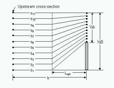
Figure: Definition sketch of assumed streamlines for low degrees of contraction.

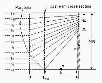
Figure: Definition sketch of assumed streamlines for high degrees of contraction.

The optimum length is defined as:

\[ L_{opt} = \frac{b}{\pi \left(1 -m'\right)}\Phi \]

Equation: Optimum bridge opening length to minimize flow contraction losses.

where

\[ m' = 1 - b/B \]

Equation: Effective width ratio, corrected for the eccentricity of the bridge opening.

\[ \Phi = \frac{1}{2}\ln\left[\left(\sqrt{\frac{8}{\varepsilon^{2}}} + 8 + \frac{3}{\varepsilon} - \varepsilon\right)\left(-\sqrt{8 + 8\varepsilon^{2}} - 3\varepsilon - \frac{1}{\varepsilon}\right)\right] - \ln\left(\varepsilon - \frac{1}{\varepsilon}\right) \]

Equation: Backwater coefficient function used in the eccentricity correction.

\[ \varepsilon = 1 + \delta + \sqrt{\delta^{2} + 2\delta} \]

Equation: Auxiliary variable used in the backwater coefficient function.

\[ \delta = \frac{2}{\tan^{2}\left[\left(1 - \dfrac{b}{2B}\right)\pi\right]} \]

Equation: Eccentricity correction factor for an asymmetrically located bridge opening.

Where:

\(b\)   The total bridge opening width excluding the piers.

\(B\)   The total width of the upstream cross section.

Effective flow length:

\[ L_{av} = \frac{1}{20}\left[\sum_{i=2}^{20}S_{i} + \frac{\left(S_{1} + S_{21}\right)}{2}\right] \]

Equation: Average length of the approach reach, from twenty cross-section spacings.

In case the optimal length is greater than the physical distance a parabola is used to describe the stream tubes. Using a coordinate system as indicated in the definition sketch for road overflow and the equation used for the right hand side of the channel is given by:

\[ x = \frac{1}{2b}\left(y^{2} - b^{2}\right) \]

Equation: Distance from the centreline for a point on the approach cross section, upstream half.

similarly the left hand side uses a parabola described by

\[ x = B - \frac{1}{2b}\left(y^{2} - b^{2}\right) \]

Equation: Distance from the centreline for a point on the approach cross section, downstream half. Expansion loss. The contraction loss from section 1 to 2 is taken into account through the use of an effective flow length as opposed to the physical distance from section 1 to section 2. No contraction or expansion loss is assumed from section 2 to 3. It is further assumed implicitly that from section 3 to section 4 only expansion takes place. If no expansion takes place the loss consists solely of the fiction loss from section 3 to 4.

The expansion loss from section 3 to 4 is computed from:

\[ h_{e} = \frac{Q^{2}}{2gA_{4}^{2}}\left[2\beta_{4} - \alpha_{4} - 2\beta_{3}\left(\frac{A_{4}}{A_{3}}\right) + \alpha_{3}\left(\frac{A_{4}}{A_{3}}\right)^{2}\right] \]

Equation: Expansion loss at the bridge exit, expressed through the velocity distribution coefficients on both sides.

\[ \beta_{3} = \frac{1}{C} \]

Equation: Velocity distribution coefficient at section 3, expressed via the discharge coefficient.

\[ \alpha_{3} = \frac{1}{C^{2}} \]

Equation: Kinetic energy coefficient at section 3, expressed via the discharge coefficient.

\[ \beta_{4} = \dfrac{\sum\left(k^{2}/a\right)}{K^{2}/A} \]

Equation: Velocity distribution coefficient at section 4, from the subsection conveyances.

\[ \alpha_{4} = \dfrac{\sum\left(k^{3}/a^{2}\right)}{K^{2}/A^{2}} \]

Equation: Kinetic energy coefficient at section 4, from the subsection conveyances.

Where:

C   Coefficient of discharge

k Subsection conveyance \(k = Mar^{2/3}\)

a   Subsection area

K   Total cross section conveyance  \(K = \sum k\)

A   Total cross section area \(A = \sum a\)

Eqs. (6.89) and (6.90) are based on a parallel channel analysis. Each parallel channel being defined through subsections. A subsection is understood as segments in series with a constant relative resistance. Further a sub-division may also be achieved through the use of markers 4 and 5. Thus for a cross section with constant relative resistance and no markers 4 or 5 the velocity coefficient is unity. Coefficient of discharge. The coefficient of discharge is a function of the bridge geometry and flow characteristics. Four main types of openings are defined the definition sketch of type I opening, vertical embankments and vertical abutments to the definition sketch of type IV opening, sloping embankments and vertical abutments. For each opening type the coefficient of discharge, C is obtained by a base coefficient C’ and a number of adjustment factors, k. The default base coefficients and adjustment factors in MIKE 1D are obtained as described by FHWA ¹.

The coefficient of discharge, C is given by:

\[ C = C' \cdot k_{F} \cdot k_{y} \cdot k_{x} \cdot k_{0} \cdot k_{e} \cdot k_{j} \cdot k_{a} \cdot k_{b} \cdot k_{d} \]

Equation: Base coefficient of discharge adjusted by the correction factors for skew, spur-dike length, eccentricity and other geometric effects.

Table: Variables in the adjusted base coefficient of discharge equation.

Adjustment factor		Type	Tabular function of:
\(C'\)	Base coefficient	All	\(m\), \(L/b\) and slope
\(k_{F}\)	Froude number	I	\(F_{3}\)
\(k_{r}\)	Corner rounding	I	\(m\) and \(r/b\)
\(k_{w}\)	Wingwall	I	\(m\), \(w/b\) and \(WW\)
\(k_{y}\)	Average depth	II	\(m\), \(\left(Y_{a} + Y_{b}\right)/(2b)\) and slope
\(k_{x}\)	Unwetted abutment	III	\(x/b\), \(L/b\) and slope
\(k_{0}\)	Wingwall	IV	\(m\), \(WW\) and slope
\(k_{e}\)	Eccentricity	All	\(K_{a}/K_{c}\)
\(k_{j}\)	Piles	All	\(m\) and \(j\)
\(k_{j}\)	Piers	All	\(m\), \(L/b\) and \(j\)
\(k_{a}\)	Elliptical spur dike angularity	All	\(m\) and \(L_{d}/b\)
\(k_{b}\)	Straight spur dike offset,	All	\(m\) and\(L_{d}/b_{d}\)
\(k_{d}\)	Spur dike length	All	\(m\) and \(L_{d}/b\)

Where:

\(m\)   Channel contraction ratio.

\(L\)   Bridge waterway flow length (length from section2 to 3).

\(b\)  Bridge opening width.

\(F_{3}\)   Froude number in downstream bridge section.

\(r\)  Radius of corner rounding.

\(w\)   Wingwall width.

\(WW\)   Wingwall angle.

\(\left(Y_{a} + Y_{b}\right)/(2b)\)       Average water level in bridge section.

\(x\)   Unwetted abutment length.

\(K_{a}/K_{c} \leq 1\)       Ratio of conveyance of the approach section on each side of the projected opening.

\(j = A_{p}/A_{3}\)    Portion of waterway blocked by piers/piles.

\(L_{d}\)  Spur dike length.

\(b_{d}\)  Spur dike offset.

The channel contraction ratio, \(m\)  is given by:

\[ m = 1 - \frac{K_{q}}{K_{1}} \]

Equation: Discharge-weighted conveyance ratio.

Where:

\(K_{1}\) The conveyance of that part of section 1 where conveys discharge can flow through the bridge opening without contraction.

\(K_{1}\) The total conveyance for cross-section 1.

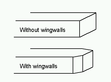
Figure: Definition sketch of type I opening, vertical embankments and vertical abutments, with or without wingwalls (after Matthai).

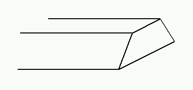
Figure: Definition sketch of type II opening, sloping embankments without wingwalls (after Matthai).

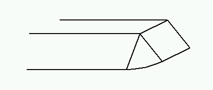
Figure: Definition sketch of type III opening, sloping embankments and sloping abutments (spillthrough) (after Matthai).

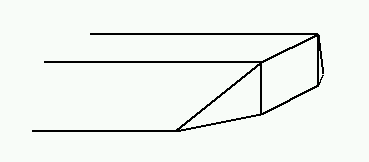
Figure: Definition sketch of type IV opening, sloping embankments and vertical abutments with wingwalls (after Matthai).

If the abutments are of different types a value of the coefficient of discharge is obtained through a weighted average:

\[ C = \frac{C_{L}K_{L} + C_{R}K_{R}}{K_{L} + K_{R}} \]

Equation: Combined discharge coefficient for left and right bridge openings, weighted by conveyance.

Where:

\(C_{L}\)  Coefficient of discharge for left abutment.

\(C_{R}\)   Coefficient of discharge for right abutment.

\(K_{L}\)  Conveyance for left side.

\(K_{R}\)  Conveyance for right side. The solution method. The method assumes that the flow through the bridge is sub-critical. Further the method is an iterative method. The bridges are pre-calculated based on a set of values for the water levels upstream and downstream. Thus for each set of water level values a discharge is to be determined. The algorithm for determining the discharge has the following steps:

1. Initial guess for the discharge.

2. Backwater calculation from section 4 to section 3.

3. Backwater calculation from section 3 to section 2 based on the result from step 2.

4. Backwater calculation from section 2 to section 1 based on the result from step 3.

5. The water level determined through step 4 is compared with the actual water level at section 1.

6. Based on the comparison in step 5 the discharge is either modified and the algorithm returns to step 2 or the algorithm terminates if the deviation is within acceptable limits.

Throughout the calculation the results are compared with critical flow. If the solution found is below critical water level or if one of the steps 2 - 4 do not converge the code defaults to critical flow at that location. Further if the maximum number of iterations (default 50) is reached without obtaining a valid solution the code defaults to critical flow at section one.

US Bureau of Public Roads (USBPR) method

The USBPR method estimates free-surface flow assuming normal depth conditions. The maximum afflux  \(H_{1}^{\text{*}}\) at section 1 (see the location of cross-sections) is here defined by:

\[ H_{1}^{*} = k^{*}\frac{\alpha_{2}V_{N2}^{2}}{2g} + \alpha_{1}\left[\left(\frac{A_{N2}}{A_{4}}\right)^{2} - \left(\frac{A_{N2}}{A_{1}}\right)^{2}\right]\frac{V_{N2}^{2}}{2g} \]

Equation: Afflux for the WSPRO spur-dike method, including the pier-loss coefficient and the velocity head redistribution term.

Where:

\(k^{\text{*}}\)  The backwater coefficient.

\(V_{N2}\)  Average velocity in bridge section at normal depth.

\(A_{N2}\) Cross section area at normal depth.

\(A_{1}\) Cross section area at section 1.

\(A_{4}\)  Cross section area at section 4.

\(g\)  Acceleration due to gravity.

\(\alpha_{1}\) Velocity distribution coefficient - Equation the velocity distribution coefficient, from the subsection conveyances at.

\(\alpha_{2}\)  Velocity distribution coefficient for normal depth.

The velocity distribution coefficient, \(\alpha_{2}\) is a function of  \(\alpha_{1}\) and the opening ratio. The opening ratio defined by

\[ M = 1 - b/B \]

Equation: Effective width ratio for the pier-loss correction.

where b is the bridge opening width and B is the width of the upstream river cross-section. In MIKE 1D the coefficient is computed from a user defined table or the pre-computed default table.

The total backwater coefficient is given by:

\[ k^{*} = k_{b}^{*} + \Delta k_{e}^{*} + \Delta k_{\phi}^{*} + \Delta k_{p}^{*} \]

Equation: Total pier-loss coefficient, combining the base, eccentricity, skew and spur-dike-length corrections.

Where:

\(k_{b}^{*}\)   Base coefficient. Tabular function of the opening ratio.

\(\Delta k_{e}^{*}\)   Eccentricity coefficient. Tabular function of the opening ratio and the eccentricity.

\(\Delta k_{\phi}^{*}\)   Skewness coefficient.Tabular function of the opening ratio and skewness angle  \(\phi\).

\(\Delta k_{p}^{*}\)   Bridge pier coefficient. Tabular function of opening ratio, the portion of waterway blocked by piers and pier type.

The eccentricity e is given by

\[ e = \frac{\text{min}\left(Q_{\text{left}}, Q_{\text{right}}\right)}{\text{max}\left(Q_{\text{left}}, Q_{\text{right}}\right)} \]

Equation: Bridge pier asymmetry measured by eccentricity of flow distribution.

where Q_left, Q_right are the ratio of discharge of the approach section on each side of the projected opening. The portion of the waterway blocked by piers is user defined an should be understood as the ratio of the pier cross sectional area to the cross sectional area of the waterway without the piers.

The coefficients are computed in MIKE 1D from user defined tables or from the pre-computed default tables.

Multiple Waterway Opening

When working with multiple openings each opening is evaluated seperately. Up- and downstream cross sections are reduced to the part found in between the stagnation points. The stagnation points are the points in the cross section where the flow splits up between the different water way openings. The default stagnation points are evaluated strictly from a geometric point of view. The default stagnation points are set so each sub cross section satisfies:

\[ B_{sub} = \frac{b}{b_{Total}}B_{total} \]

Equation: Width of a submerged sub-opening, proportional to its share of the total waterway width.

Where:

\(B_{sub}\)   Width of sub cross section.

\(b\)   Bridge opening width from marker 1 to 3

\(b_{Total}\)   Total width of all bridge openings.

\(B_{Total}\)  Total width of cross section from marker 1 to 3.

The user can set the stagnation points if desired.

Pressure Flow, Federal Highway Administration method

During significant contact of the water surface with the girders of the bridge structure, free-surface flow cannot exist and pressure flow is etablised.

Fully Submerged Orifice flow

Discharge through the fully submerged bridge opening is computed by:

\[ Q_{orifice} = C_{D}A_{2}\sqrt{2g\left(h_{1} - h_{f12} + h_{v1} - h_{3}\right)} \]

Equation: Discharge through a culvert acting as a submerged orifice.

Where:

A₂   Flow area in the bridge opening.

g   Acceleration due to gravity.

h₁   Water level in the upstream cross section.

h_v1   Velocity head at cross-section 1.

h₃   Water level in the downstream bridge section.

h_f12   The friction loss from the upstream cross section to the upstream bridge section.

C_D   Discharge coefficient (default 0.8).

The friction loss is expressed as

\[ h_{f12} = \frac{L_{12}Q_{t}^{2}}{K_{1}K_{2}} \]

Equation: Friction loss between sections 1 and 2 of the culvert.

where the flow length is either the effective length or the physical length depending on the free bridge modelling method. The discharge Q_t is the total discharge including possible overflow. The conveyance at sections 1 and 2 are calculated as defined in eqs. (6.69)-the total flow area as sum of subsection flow areas.

The water level in sections 2 is given by

\[ h_{2} = h_{1} - h_{f12} \]

Equation: Water level at section 2, after friction losses from section 1.

and the water level at section 3 is obtained from solving the appropriate version of the energy equation from section 4 to section 4.

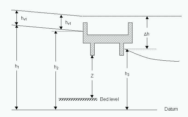
Figure: Definition sketch for submerged orifice flow.

Orifice flow

If the water surface is only in contact with the bridge bottom on the upstream side of the bridge the discharge is found through:

\[ Q = C_{D}A_{2}\sqrt{2g\left(Y_{2} - Z/2 + h_{v1}\right)} \]

Equation: Discharge through a culvert flowing full, orifice equation referenced to the culvert soffit.

Where:

\(C_{D}\)   Discharge coefficient. Tabular function of \(Y_{2}/Z\).

The quantities are defined in the definition sketch for orifice flow note that the bed level is defined as

\[ \text{Bed Level} = b_{bottom} - Z \]

Equation: Bed level used for the culvert's outlet control calculation.

where \(b_{bottom}\) is the bridge bottom level and \(Z = A_{2}/B_{2}\).The quantity A₂ being the area at the opening and B₂ is the width at the bridge bottom level.

Equation the discharge through a culvert flowing full, orifice equation referenced to the may be rewritten as

\[ c_{orifice}A\sqrt{2g\left(h -\text{max}\left(h_{p}, h_{ds}\right)\right)} \]

Equation: Discharge through submerged bridge opening as orifice flow from upstream to downstream energy head.

which is a form equivalent to equation the discharge through a culvert acting as a submerged orifice. Note that the discharge coefficient in the two equations are different. To ensure a smooth transition from free orifice flow to submerged orifice flow a linear transition is made on the discharge coefficient from free to submergence. That is for water levels below the level  \(b_{bottom} - Z/2\) the free submergence coefficient is used whereas as the water level increases downstream and the orifice slowly becomes drowned the coefficient changes continuously into the fully submerged value. Further to avoid an abrupt change in the solution when the downstream water level reaches the bottom of the bridge the orifice equation is modified as

\[ Q = C_{D}A_{2}\sqrt{2g\left(Y_{2} -\frac{Z}{2} + h_{v1}\right)} \]

Equation: Discharge through a bridge opening as a submerged orifice with tailwater correction.

where the modified downstream water level \(\hat{h}_{3}\) is given by

\[ \hat{h}_{3} = \min\left(h_{3}, b_{bottom} - Z/2\right) \]

Equation: Effective downstream water level for outlet control, capped at the culvert soffit.

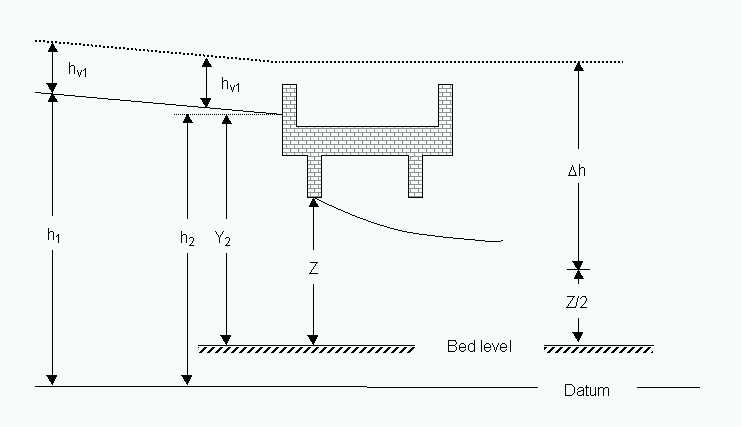
Figure: Definition sketch for orifice flow.

Road overflow, Federal Highway Administration method

When the water surface elevation exceeds the top bridge level the top part of the bridge is assumed to function as a weir. The discharge for the overflow part is computed using a weir formula:

\[ Q = k_{t}C_{f}B_{W}H^{3/2} \]

Equation: Discharge for a culvert flowing under inlet control.

Where:

\(H\)  Total head for weir flow with respect to bridge top level (see the definition sketch for road overflow).

\(k_{t}\)  Adjustment factor due to possible submergence from downstream water level. Tabular function of tail water level \(h_{t}\) and total head  \(H\).

\(C_{f}\)  Coefficient of free discharge. Tabular function of water depth on the structure \(h_{s}\), the crest length in the flow direction  \(L_{R}\) and the total head \(H\).

\(B_{W}\)   Width of overflow part.

The submergence adjustment factor \(k_{t}\) depends on the ratio of minimum elevation along the top of the embankment   \(h_{t}\)to the total head for weir flow  \(H\).

The total head for weir flow is given by:

\[ H = h_{1} + h_{v1} - L_{12}\frac{Q_{Tot}^{2}}{K_{1}^{2}} - h_{weir} \]

Equation: Upstream energy level required to pass the design discharge, including the approach velocity head and friction/weir losses.

Where:

\(h_{1}\)  Water level at cross section 1.

\(h_{v1}\)  Velocity head at cross-section 1.

\(L_{12}\)  Distance between section 1 and section 2.

\(Q_{Tot}\)   Total discharge including under flow through the bridge.

\(K_{1}\)  Conveyance for cross-section 1.

\(h_{weir}\)  Crest level.

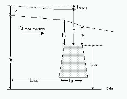
Figure: Definition sketch for road overflow.

Trouble shooting for bridge structures

During the simulation the discharge through a bridge is determined from a pre-calculated table. Each value in the table is found by an iteration process. Using a pre-calculated table decreases the calculation time.

Instability

For bridge structures a number of factors can result in instabilities.

Time step: In most cases it is helpful to decrease the MIKE 1D time step.

Delta: Delta is a default value in the HD editor. Increasing delta reduces instabilities. The delta value controls the time centering in the scheme.

Bridge preprocessing: To speed up simulations the bridges are preprocessed initially at simulation start. The generated H-Q-H tables are saved into files named using the bridge ID. In the present version the files are exported in the dfs2 format which can be readily viewed using standard tools within MIKE Zero. It is recommended to evaluate these files for consistency. Note that non-smooth H-Q-H surfaces may be caused by abrupt changes in bed friction or geometry.

River (MIKE 11 / MIKE HYDRO)

Further consult MIKE11.ini for further capabilities with regards to bridge preprocessing.

Results

‘Curtains’: ‘Curtains’ in the result curve may be a result of the pre-calculated table. Increasing the resolution in the pre-calculated table will generally decrease the ‘curtain’ size.

River (MIKE 11 / MIKE HYDRO)

BRIDGE_TABLE_GRID_UPSTREAM and BRIDGE_TABLE_GRID_DOWNSTREAM in MIKE11.ini may be used to specify a different resolution for the water levels used for the pre-calculated tables. The default value is 0.1 meters. The value is given in meters.

---

1. Federal Highway Administration: Bridge Waterways Analysis Model: Research Report, Report No. FHWA/RD-86/108, July 1986, Washington D.C. ↩

2. Hamil, L.: Bridge Hydraulics. E & FN Spon, 1999. ↩