Kinematic Wave Surface Runoff Model
Kinematic Wave Surface Runoff Model
Concept
The concept of this surface runoff computation is founded on the kinematic wave computation. The surface runoff is computed as flow in an open channel, taking in to account the gravitational and friction forces only. The amount that runs off is controlled by the various hydrological losses and the size of the actually contributing area.
The shape of the runoff hydrograph is controlled by the catchment parameters length, slope and roughness of the catchment surface. These parameters form a base for the kinematic wave computation using the Manning equation.
The catchment is divided into five sub-catchments that have different permeability properties of the surface. The five surface types are:
Table: Permeability properties of sub-catchment surfaces.
| Permeability | Surface type |
|---|---|
| Impervious | Steep Flat |
| Pervious | Small Medium Large |
Only relevant processes are modelled on each surface type. The model applies different hydrological parameters for each of the surface types. The total runoff is computed as the sum of these sub-catchments.
Input data
Model specific data
Length [m] is defined by the catchment shape, as the flow channel. The model assumes a prismatic flow channel with rectangular cross section. The channel bottom width is computed from catchment area and length.
The default value is 10 m.
Slope [-] is the average slope of the catchment surface, used for the runoff computation according to Manning equation.
The default value is 1.
Surface type areas [-] represent the fractions of the catchment surface belonging to each surface types.
The default value depends on the surface type (see the default hydrological parameters for Kinematic wave surface runoff model).
Hydrological Parameters - Soil Infiltration
Wetting loss [m] is a one-off loss, accounting for wetting of the catchment surface.
The default value for all surface types is 5.00E10-5 m.
Storage loss [m] is a one-off loss, which defines the precipitation depth required for filling the depressions on the catchment surface prior to occurrence of runoff.
The default value depends on the surface type (see the default hydrological parameters for Kinematic wave surface runoff model)
Start infiltration rate [m/s] defines the maximum rate of infiltration (Horton) for the specific surface type.
The default value depends on the surface type (see the default hydrological parameters for Kinematic wave surface runoff model).
End infiltration rate [m/s] defines the minimum rate of infiltration (Horton) for the specific surface type.
The default value depends on the surface type (see the default hydrological parameters for Kinematic wave surface runoff model).
Wet Horton Exponent [s-1] is time factor “characteristic soil parameter”. It determines the dynamics of the infiltration capacity rate reduction over time during wet period. The actual infiltration capacity is made dependent of time since the rainfall start only.
The default value depends on the surface type (see the default hydrological parameters for Kinematic wave surface runoff model).
Dry Horton Exponent [s-1] is a time factor used in the “inverse Horton's equation”, defining the rate of the soil infiltration capacity recovery after a rainfall, i.e. in a drying period.
The default value depends on the surface type (see the default hydrological parameters for Kinematic wave surface runoff model).
Manning’s number [m1/3s-1] describes roughness of the catchment surface, used in hydraulic routing of the runoff (Manning's formula).
The default values depend on the catchment surface category (see the default hydrological parameters for Kinematic wave surface runoff model).
Table: Default hydrological parameters for Kinematic wave surface runoff model, Impervious and Pervious.
| Parameter | Steep imp. | Flat imp. | Small per. | Medium per. | Large per. |
|---|---|---|---|---|---|
| Area fraction (-) | 0 | 0.4 | 0 | 0 | 0.6 |
| Wetting (m) | 5.00E-5 | 5.00E-5 | 5.00E-5 | 5.00E-5 | 5.00E-5 |
| Storage (m) | - | -6.00E-4 | 1.00E-3 | 1.00E-3 | 2.00E-3 |
| Start inf. rate (m/s) | - | - | 8.00E-7 | 8.00E-7 | 2.00E-5 |
| End inf. rate (m/s) | - | - | 8.00E-7 | 8.00E-7 | 3.00E-6 |
| Wet exponent (s-1) | - | - | 0 | 0 | 1.50E-3 |
| Dry exponent (s-1) | - | - | 0 | 0 | 3.00E-5 |
| Manning (m1/3s-1) | 80 | 70 | 30 | 30 | 12 |
Runoff computations
The model computations are based on the volume continuity and the kinematic wave equations.
The first step is the calculation of the snow storage if relevant, then the effective precipitation intensity. The effective precipitation intensity is the precipitation which contributes to the surface runoff, i.e. when the losses have been taken into account (evaporation, infiltration...)
Next, the hydraulic routing based on the kinematic wave formula (Manning) and volume continuity is applied. The sketch with schematics of the model computation is shown in the simulated processes in Kinematic wave surface runoff model.
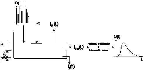
Figure: The simulated processes in Kinematic wave surface runoff model.
Snow storage computation
Snow can accumulate when the temperature is inferior or equal to zero degrees Celsius (\(T \leq 0^{\circ}\text{C}\) ). During warmer periods, when temperature exceeds zero degrees Celsius (\(T > 0^{\circ}\text{C}\)), the snow storage melts at a rate given by the snow melt coefficient. The snow storage computation will be performed only if a temperature time series is provided for the catchment.
During storing periods, or \(I_w\) the snow will accumulate without limit. If the temperature is below zero degrees Celsius, it is assumed that the entire rainfall will be stored as snow.
During melting periods, or T>0°C the snow will melt and therefore contributes to the surface runoff at rate given by the snow melt coefficient.
The snow module is the first process occurring after rainfall, therefore all others losses will be computed afterwards.
Effective precipitation computation
The simulated hydrologic processes account for various losses calculated - evaporation, wetting, infiltration and surface storage -according to the conventions and equations presented below. The remaining precipitation is called effective precipitation, defined generally as:
Equation: Effective precipitation, defined as the actual precipitation reduced by the evaporation, wetting, infiltration and surface storage losses.
Where:
Table: Variables used in the effective precipitation equation.
| \(I(t)\) | Actual precipitation at time t |
| \(I_E(t)\) | Evaporation loss at time t. It should be noted that the evaporation loss for the catchment is accounted only if an evaporation time series in provided |
| \(I_W(t)\) | Wetting loss at time t |
| \(I_I(t)\) | Infiltration loss at time t |
| \(I_S(t)\) | Surface Storage loss at time t |
The individual terms in the loss equation are fundamentally different, as some terms are continuous where others are discontinuous. If the calculated loss is negative, it is set to zero. The losses have a dimension of velocity [LT-1].
The actual precipitation, I(t), is assumed to be uniformly distributed over the individual catchments. Otherwise, it may vary as a random time function.
The evaporation, IE(t), is a continuous loss that is normally of less significance for single event simulations. However, on a long-term basis, evaporation accounts for a significant part of hydrological losses. If included in the computation, the evaporation is the first part subtracted from the actual precipitation, according to the following:
Equation: Evaporation loss, limited by the potential evaporation and the availability of ponded water.
Where:
Table: Variables used in the evaporation loss equation.
| \(I(t)\) | Actual precipitation at time t |
| \(I_E(t)\) | Evaporation loss at time t |
| \(I_{PE}(t)\) | Potential evaporation at time t |
| \(y(t)\) | Accumulated depth at time t |
If the actual evaporation is not explicitly specified in the simulation (i.e. Evaporation process activated – see INI file parameters – and evaporation time series specified), only a decay rate will be applied during dry periods.
The wetting, IW(t), is a discontinuous loss. When the precipitation starts, a part of the precipitation is used for wetting of the surface if the surface is initially dry. The model assumes that the precipitation remaining after subtraction of the evaporation loss is used for wetting of the catchment surface. When the surface is wet, the wetting loss, IW, is set to zero. This is summarised in the following expression:
Equation: Wetting loss, applied until the wetting depth is reached.
Where:
Table: Variables used in the wetting loss equation.
| \(I(t)\) | Actual precipitation at time t |
| \(I_E(t)\) | Evaporation loss at time t |
| \(I_W(t)\) | Wetting loss at time t |
| \(y_w\) | Wetting depth |
| \(y(t)\) | Accumulated depth at time t |
The infiltration, II(t), is the water loss to the lower storage caused by the porosity of the catchment surface. It is assumed that the infiltration starts when the wetting of the surface has been completed. The infiltration loss is calculated according to the following relation:
Equation: Infiltration loss, capped by the maximum infiltration capacity and zero once wetting depth is exceeded.
Where:
Table: Variables used in the infiltration loss equation.
| \(I_I(t)\) | Infiltration loss at time t |
| \(I_H(t)\) | Horton’s infiltration at time t |
| \(y_w\) | Wetting depth |
| \(y(t)\) | Accumulated depth at time t |
The infiltration is a complex phenomenon, dependent on the soil porosity, moisture content, groundwater level, surface conditions, storage capacity, etc. The model calculates the infiltration loss capacity using the well-known Horton's equation, per default in its original form:
Equation: Horton's equation for the infiltration capacity, original form.
Where:
Table: Variables used in Horton's infiltration capacity equation.
| \(I_H(t)\) | Infiltration loss calculated according to Horton |
| \(I_{Imax}\) | Maximum infiltration capacity (after a long dry period) |
| \(I_{Imin}\) | Minimum infiltration capacity (at full saturation) |
| t | Time since the start of the storm |
| ka | Time factor (characteristic soil parameter) for wetting conditions |
The Horton's equation in its original form the horton's equation for the infiltration capacity, original form yields in realistic results only if applied to events for which the rainfall intensity always exceeds the infiltration capacity. However, typical values for infiltration capacity parameters IImax and IImin are often greater than typical rainfall intensities. Thus, when Equation the horton's equation for the infiltration capacity, original form is used, with infiltration capacity IH being the function of time only, IH will decrease even if rainfall intensities are very small. In other words, this results in a reduction in infiltration capacity regardless of the actual amount of water entering the soil. This problem is solved by implementing the integrated form of the Equation the horton's equation for the infiltration capacity, original form:
Equation: Integrated form of Horton's equation, giving the cumulative infiltration up to the equivalent time.
Where:
Table: Variables used in the integrated form of Horton's equation.
| ICUM(tp) | A cumulative infiltration (m) at time tp, i.e. the area under the Horton's curve |
This assumes that the actual infiltration has been equal to the infiltration capacity at any time within the period 0->t. Since this is only the case for rainfall intensities higher than the infiltration capacity, this needs to be corrected as:
Equation: Cumulative infiltration at the elapsed time, from the actually occurred infiltration.
i.e. the cumulative infiltration at the elapsed time t is calculated using the actually occurred infiltration.
At any elapsed time t, the two equations the integrated form of Horton's equation, giving the cumulative infiltration up to and the cumulative infiltration at the elapsed time, from the actually occurred can be used to determine the “equivalent” time tp. This is done iteratively, since equation the integrated form of Horton's equation, giving the cumulative infiltration up to cannot be solved explicitly for tp.
The time tp on cumulative Horton's curve will always be less or equal than the actually elapsed time, implying that the available infiltration capacity at time tp will be greater than or equal to that given by the equation the horton's equation for the infiltration capacity, original form. By these means, the infiltration capacity has been made a function of actual water infiltrated and not just a function of time.
Per default, the program is set to “standard” Horton's equation. Application of a “standard” Horton's equation the horton's equation for the infiltration capacity, original form or its integrated form (Equations the integrated form of Horton's equation, giving the cumulative infiltration up to and the cumulative infiltration at the elapsed time, from the actually occurred) is controlled par the parameter Integrated Horton.
MIKE 11 note: the integrated Horton form of the equation is not available from MIKE 11 interface, so only its “normal” form can be used.
In the dry period following the rainfall, the infiltration capacity is gradually recovered to the initial value, using an inverse form of the Horton's equation:
Equation: Recovery of the infiltration capacity during the dry period following rainfall, inverse form of Horton's equation.
Where:
Table: Variables used in Horton's infiltration capacity recovery equation.
| \(I_H(t)\) | Infiltration loss capacity calculated according to Horton |
| \(I_{Imax}\) | Maximum infiltration capacity (after a long dry period) |
| \(I_{IT}\) | Infiltration capacity at the threshold between the wetting and drying period |
| t | Time since the start of the recovery process |
| kh | Dry Horton Exponent, the time factor (characteristic soil parameter) for drying conditions |
The surface storage, IS(t), is the loss due to filling the depressions and holes in the terrain. The model begins with the surface storage calculation after the wetting process is completed. The surface storage is filled only if the current infiltration rate is smaller than the actual precipitation intensity reduced by evaporation. The actual surface storage loss is calculated according to the following:
Equation: Surface storage loss, filling the terrain depressions once the wetting and infiltration losses are satisfied.
Where:
Table: Variables used in the surface storage loss equation.
| \(I(t)\) | Precipitation intensity at time t |
| \(I_S(t)\) | Surface storage loss at time t |
| \(I_I(t)\) | Infiltration loss at time t |
| \(I_W(t)\) | Wetting loss at time t |
| \(I_E(t)\) | Evaporation loss at time t |
| \(y_w\) | Wetting depth |
| \(y_s\) | Surface storage depth |
| \(y(t)\) | Accumulated depth at time t |
Surface Runoff routing computation
The runoff starts when the effective precipitation intensity is larger than zero. The hydraulic process is described with the kinematic wave equations for the entire surface at once. This description assumes uniform flow conditions on the catchment surface, i.e. equal water depth over the entire surface of certain category.
This type of runoff model is also called a non-linear reservoir model.
The surface runoff at time t is calculated as:
Equation: Surface runoff, kinematic wave (Manning) formula.
Where:
Table: Variables used in the kinematic wave surface runoff equation.
| M | Manning’s number |
|---|---|
| M | Manning’s number |
| B | Flow channel width, computed as: B [m] = A [m 2 ] / L [m] |
| I | Surface slope |
| Runoff depth at time t |
The depth yR(t) is determined from the continuity equation:
Equation: Continuity equation determining the runoff depth.
Table: Variables used in the continuity equation for runoff depth.
| Ieff | Effective precipitation |
| A | Contributing catchment surface area |
| dt | Time step |
| \(dy_R\) | Change in runoff depth |
Hydrological losses depending on surface type
The Kinematic Waves Surface Runoff Model distinguishes between up to 5 different catchment surface types. This is practically handled by the model so that the individual catchment is split into up to five sub-catchments, each with the area according to the specified percentages for specific surface categories.
For each surface type, only relevant processes are simulated. An overview of the processes associated with different surface types is shown in the processes included for various types of catchment surface.
Table: Processes included for various types of catchment surface.
| Surface Type | Hydrological Loss Simulated |
|---|---|
| Impervious Steep | Evaporation Wetting |
| Impervious Flat | Evaporation Wetting Storage |
| Pervious small | Evaporation Wetting Infiltration Storage |
| Pervious medium | Evaporation Wetting Infiltration Storage |
| Pervious large | Evaporation Wetting Infiltration Storage |
The model treats every area with different surface category as a sub-catchment, and the runoff computations are performed individually. The total runoff from the entire catchment is obtained then as a sum of runoffs from up to five different sub-catchments.
Definition of the sub-catchment geometry
The length and width for each sub-catchment (sub-area) are calculated so that the length/width ratio for each sub-area is kept equal to the length/width ratio of the corresponding catchment. Based on the information for the whole catchment and the principle of constant length/width ratio, equivalent values of the runoff width and length are computed for all sub-areas, as illustrated in the example below (the sub-catchments with total area = 833 m2).
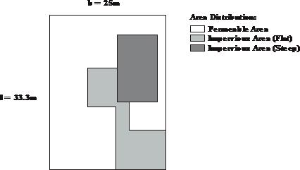
Figure: Sub-catchments with total area = 833 m2.
The ratio between the catchment length and width in the given example corresponds to 1.33. 15% of the total area is impervious roof surface corresponding to 125 m2. Hence the runoff length is 12.9 m and the runoff width is 9.7 m for this surface type, as 12.9 * 9.7 = 125 and 9.7 * 1.33 = 12.9.
Multiple-Event Simulations
If the Kinematic Wave Surface Runoff Model is used for a continuous simulation of multiple rainfall events, a special solution has been applied for the simulation of dry periods between the consecutive events. The solution accounts for the following phenomena:
Recovery of the soil infiltration capacity
According to Horton equations, the soil infiltration capacity is getting reduced as the soil gets more saturated by rain. In dry periods, an inverse process occurs, with gradual recovery of the infiltration capacity. Computation of both processes is detailed in Section 7.4.3.
As a consequence of wet and dry period alternation in a multiple event simulation, the model alternates between the two computation modes. Switching to the “dry” mode is triggered by the exhaustion of all water available for infiltration. Consecutively, switch to the “wet” mode at the start of a new rain event.
Recovery of the initial loss capacity during dry intervals
The occurrence of the initial loss at the beginning of each simulated event is modelled in accordance with reality. During dry periods, the initial loss capacity will be recovered if no evaporation time series has been provided. In other words, the recovery of the initial loss capacity is meant to replaces the actual evaporation.
In this context, start of a dry period is defined if three conditions are fulfilled simultaneously:
- No rainfall: all connected rain gauges show no rain, i.e. the rainfall intensity is null
- No infiltration: the infiltration has stopped in the catchment (and not necessary in all catchment like it is done in MOUSE)
- No runoff: the runoff from the catchment included in the simulation has fallen below the “low flow” limit. The threshold can be controlled through the parameter RUNOFF_B_LOW_FLOW in the INI file (see relevant documentation for reference).
At the start of a dry period, the initial loss storage would appear fully or partially filled up. For flat impervious surfaces, the full initial loss storage would contain the water used for wetting and filling of the surface storage, while for all other surface types only wetting loss will apply. The latter case, i.e. partially filled storage would apply for small events with the total depth smaller than the corresponding initial loss storage capacity.
Recovery of the initial loss capacity, i.e. the process of surface drying is simulated as a constant “decay” rate, which replaces the actual evaporation. As a consequence of the recovery process, the initial loss storage would be fully or partially emptied, which depends on the actually applied loss recovery rate and the duration of the dry period.
The initial loss recovery rate can be controlled through RUNOFF_B_INITLOSS_RECOVER found in the INI file (see relevant documentation for reference).
The recovery process is only activated during dry periods, i.e. the evaporative action during rain events is neglected. Note that if actual evaporation process is activated, the recovery process is suppressed and evaporative action is activated throughout the simulation period.
In order to speed up the simulation, dry periods between events are per default simulated with longer time steps. The dry period time step is controlled through the parameter RUNOFF_B_LOW_FLOW found in the INI file (see relevant documentation for reference). Switching to different time step in dry period can be suppressed by setting the parameter RUNOFF_B_Variable_dT found the ini file (see relevant documentation for reference). This functionality is not available from MIKE 11.