Super Critical Flow

The Saint-Venant equations are accurate in the fully dynamic wave approximation only for subcritical flow conditions, i.e. for Froude numbers less than 1. In supercritical flow conditions, a more stable and accurate flow description is obtained by suppressing inertia forces in the conservation of momentum equation (the second term in equation (4.1b)). Even though this approach increases stability for supercritical flow, it should be noted that the 1D solution scheme is more accurate at low Froude numbers (less than 1) than at higher Froude numbers.

Convection suppression factor

The characteristics of the Saint-Venant equations are given by

\[ C_{1,2} = \frac{q}{A_{fl}} \pm \sqrt{\frac{g A_{fl}}{b_s}} = \frac{q}{A_{fl}} \left( 1 \pm \frac{1}{F} \right) \]

Equation: Characteristic wave speeds in Saint-Venant equations related to Froude number.

For F > 1 the characteristics are both positive, implying that the Saint-Venant equations take two upstream boundary conditions, and for F = 1 the solution becomes singular. The numerical algorithm adopted is based on a staggered computational grid and cannot accommodate two boundary conditions at the same boundary and cannot handle a singular solution. To avoid these situations a modified momentum equation is implemented:

\[ \frac{\partial q}{\partial t} + \beta \frac{\partial\left(\alpha \frac{q^2}{A_{fl}}\right)}{\partial x} + g A \frac{\partial h}{\partial x} + g A f_r q |q| = f \]

Equation: Modified momentum equation for supercritical flow with convection suppression term dependent on Froude number.

where \(\beta\) is a convection suppression term dependent on the Froude number. The default formulation is

\[ \beta = \begin{cases} 1 - F^2 & \text{for } F \leq 1 \\ 0 & \text{for } F > 1 \end{cases} \]

Equation: Froude-number-dependent convection suppression factor to stabilize solutions at high flow speeds.

This ensures excellent stability properties of the numerical solution and is sufficiently accurate for most flood routing studies, where generally the Froude numbers are relatively small and the resolution used is coarse (\(\Delta x \gg h\)). The suppression term is shown in the Convection suppression term (beta) as a function of the Froude number.

For water surface profiles with high a Froude number and small space steps (\(\Delta x\)= O (water depth)) an alternative formulation has been implemented:

\[ \beta = \begin{cases} 1 & \text{for } F < a \\ 1 / (F + 1 - a)^b & \text{for } F > a \end{cases} \]

Equation: Alternative convection suppression formulation for high Froude numbers.

For the default value of a and b (a=1 and b=2) the two characteristics never have the same sign; when \(F<1\) they have different signs, and when \(F\geq1\) then one is zero. The variation of b is shown in the Convection suppression term (beta) as a function of the Froude number.

The alternative formulation is somewhat less stable than the default, Equation the froude-number-dependent convection suppression factor to stabilize solutions at, and therefore requires the application of a smaller time step for high Froude numbers. The solution is, however, considerably more accurate for high Froude numbers. Various tests have shown that the alternative formulation performs well for the transition from sub- to supercritical flow, whereas hydraulic jumps are less accurate.

Note that a and b can be adjusted and do not necessarily have to be set at a=1 and b=2. However, the solution scheme is unstable if the suppression factor b lies to the right of the dashed curve shown in the Convection suppression term (beta) as a function of the Froude number. Thus a=0.5 and b=2 can be applied, but a=2 and b=2 cannot.

The same factor (\(\beta\)) is used to gradually centre the evaluation of the differentials upstream as the flow approaches supercritical conditions.

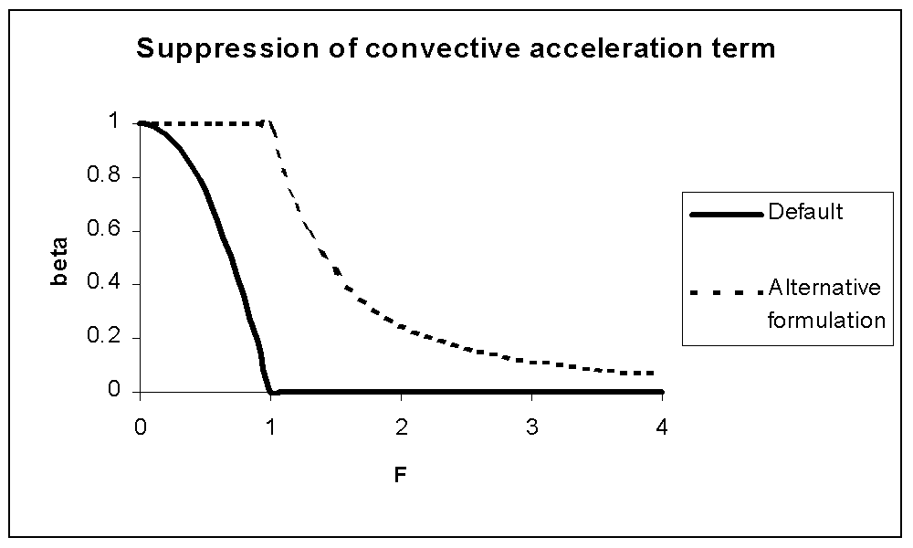
Figure: Convection suppression term (beta) as a function of the Froude number, showing gradual reduction of the convection term during transition to supercritical flow.

Effect of convection suppression on energy heads

As discussed, when the solution scheme approaches critical conditions the convective momentum term is gradually reduced. The suppression factor b varies from 1 (full convective term) to 0 (no convective term) according to the Froude number.

The b factor also modifies the energy calculation, thus energy head at any location in a model is affected. This means that when velocities are high (when the convective term is significant), the energy head is significantly affected by the value of beta. This can be seen in a profile plot of energy levels along a river reach, which shows that energy is not conserved and varies according to velocity.