Dambreak

A dambreak structure is a dam in which a breach can develop. The flow through a dam breach may be described in MIKE 1D through the use of the energy equation or alternatively through a calculation method as implemented in the National Weather Services (NWS) DAMBRK program. In the following the two methods are presented separately.

A dambreak structure consists of two underlying structures: A structure representing the flow over the crest (crest flow structure) and a structure representing the breach of the dam. The breach can be modelled in two different ways: As a failure of the crest (breach failure) or as piping failure of the dam (pipe failure) followed by breach failure.

Failure moment

The user may choose three different definitions of the failure moment, namely

• Time in the form of a historic date and time.
• Hours from start of simulation. The user specifies a time span in hours before the dam breaches.
• A reservoir water level. The reservoir water level is defined as the greatest of the water level on either side of the dam.

Energy equation based dam breach modelling

The flow at the dambreak structure is quite similar to a broad crested weir, but there are two differences:

1. The shape of the dam changes with time, i.e. the breach increases and the dam crest is shortened. As a consequence the critical flow characteristics (Q-h) relationship of the crest and of the breach cannot be calculated in advance.

2. the Q-h relationship for the dam crest and the breach are different. Therefore the flow over the crest and the flow through the breach are calculated separately, see the combined flow over breach and crest.

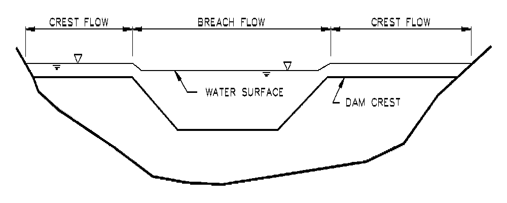
Figure: Combined flow over breach and crest.

Trapezoidal breach geometry

During the development of the breach the trapezoid increases in size and changes shape.

The initial breach shape is described by three parameters as shown in the parameters of the breach geometry:

• Level of the breach bottom (HB)
• Width of the breach bottom (WB)
• Side slope of the breach (SS) (horizontal divided by vertical lengths). The left side slope and the right side slope are equal

The development of the breach can either be specified as a known function of time, or it can be calculated from the sediment transport capacity of the breach flow.

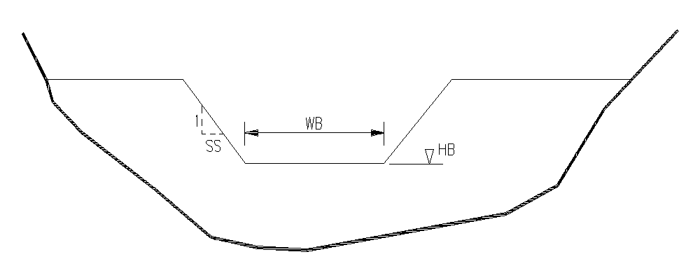
Figure: The parameters of the breach geometry.

Known geometry breach development

If this method is used, then the parameters of the breach are given as a time series in a boundary. The time is relative to the start of the breach. Between the specified times the parameters are linearly interpolated as shown in the breach is specified for example at times 0h and 1h for the trapezoidal case. The breach bottom level must not be above the crest level.

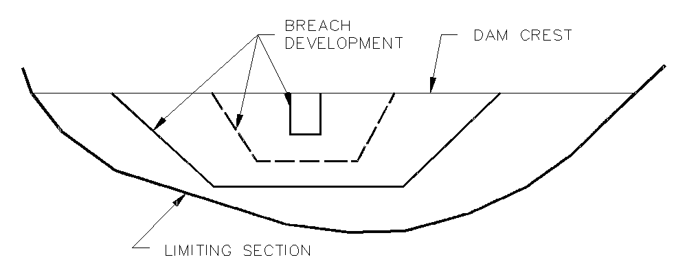
Figure: The breach is specified for example at times 0h and 1h. The dashed line would be the linear interpolation for time 0.5h.

Erosion based breach development using the energy equation

If this mode is used, the initial and the final breach shape must be specified. The increase of the breach during a time step is calculated from the conditions in the breach itself. The Engelund-Hansen sediment transport formula is used (see the MIKE reference manual for Non-cohesive sediment transport module) to calculate the sediment transport in the breach.

As a first step, the flow resistance in terms of the total dimensionless shear stress is calculated, based on the Engelund formulation. This is then compared to the critical shear stress (the Shield’s Criterion, defined by the user). If the computed shear stress is greater than the critical stress, then the sediment transport is calculated, otherwise it is set to zero.

The sediment transport rate, q_t, calculated from the Engelund-Hansen formula is in terms of m²/s per metre-width of pure sediment only, and this must then be related to a change in bed (i.e. breach) level. It is assumed that the breach remains horizontal. From the given upstream and downstream slopes, the length of the breach in the flow direction, L_b, may be calculated. By application of the sediment continuity equation in the breach, the change in breach level dH_b in a time interval dt is given as:

\[ \frac{\text{d}H_{b}}{\text{d}t} = \frac{q_{t}}{L_{b}\left(1 -\epsilon \right)} \]

Equation: Rate of change of breach level from sediment continuity accounting for porosity.

where,

H_b    is the breach level

q_t    is the sediment transport rate (m²/s)

e    is the porosity of the sediment

L_b    is the breach length in the direction of flow

t    is time

Modelling the variation of the width of the breach perpendicular to the flow direction is more difficult to relate to the classical theories of sediment transport. This is because the theories for bed load and suspended load do not apply to the development of a wall boundary layer along the often very steep side walls of the breach. As an approximation, the sediment transport at the sloping walls is assumed to be proportional to that in the central part of the breach. The coefficient of proportionality, x, (side erosion index) relates the increase in breach width, W_b, to depth as:

\[ \frac{\mathrm{d}W_{b}}{\mathrm{d}H_{b}}~=~2x \]

Equation: Rate of dam breach widening with respect to breach depth for erosion calculations.

Generally, the side erosion index is in the order of 0.5-1.0.

Erosion Based Piping Failure

An erosion based failure of a dam may be initially started by piping failure. In this case a flow forms through the dam wall. Erosion of the soil along the “pipe” causes the pipe to enlarge and the flow to increase. Eventually the dam will collapse into the void created by the piping failure erosion.

This failure scenario is modelled as an option in the erosion based breach development, i.e. there are two options for the initial failure process:

1. Initial failure by overtopping.

2. Initial failure by piping (after collapsing the erosion process returns to that of overtopping as described above).

The assumptions adopted for the piping failure are:

• The shape of the pipe is circular.
• The pipe is horizontal.
• The pipe must always be running full.

The location of the pipe centre in the dam cross section must be within the final breach shape and, if specified, the limiting section shape. When the circumference of the pipe extends outside these shapes, the hydraulic parameters are based on a reduced cross section as illustrated in the adjustment of a pipe cross section.

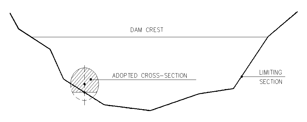
Figure: Adjustment of a pipe cross section.

The point of collapse is defined by a ratio, which is specified by the user, of the pipe diameter to the distance between the dam crest and the pipe soffit as illustrated in the definition of piping failure collapse ratio. Once this ratio is exceeded part of the dam is collapsed to form a breach.

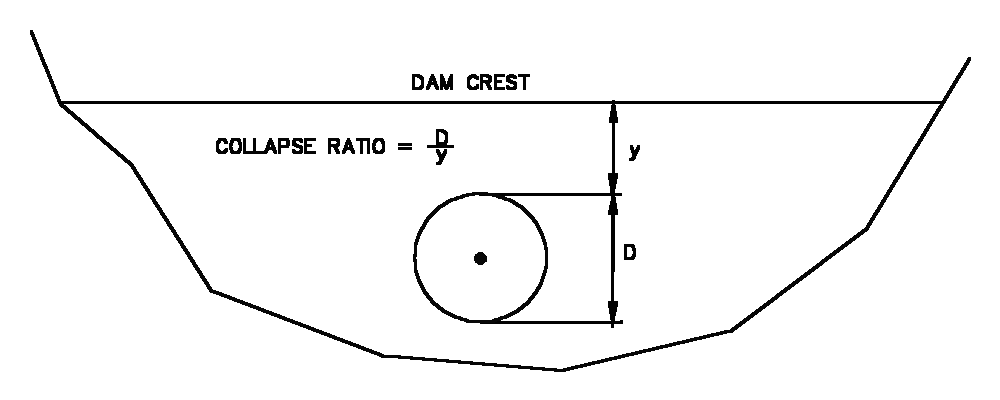
Figure: Definition of piping failure collapse ratio.

The shape of the breach is illustrated in the breach shape after collapse. The bottom width is first set equal to the pipe diameter and the breach level to the pipe invert. Not all of the collapsed material will typically be carried out without depositing on the bed of the breach. This is accounted for by a volume loss coefficient, f_lost, which is the fraction of material assumed to be washed out immediately after collapse. The remaining material is evenly distributed on the breach bed as shown in the breach shape after collapse.

These calculations are made using cross section areas, not volumes, therefore, the length of the breach and consequently the upstream and downstream slopes of the dam faces are not taken into account.

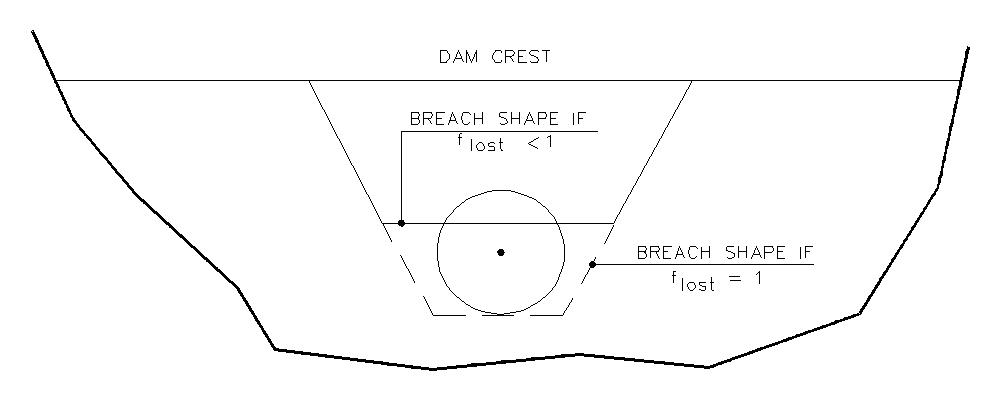
Figure: Breach shape after collapse.

Other parameters required are the initial diameter of the pipe at the start of failure and the pipe roughness, k_s, which is used to calculate the Darcy friction factor, f, according to

\[ \frac{1}{\sqrt{f}}~=~2\mathrm{log}_{10}\!\left(\frac{12R}{k_{s}}\right) \]

Equation: Darcy friction factor from pipe roughness and hydraulic radius using Colebrook-White equation.

where, R is the hydraulic radius.

The discharge, Q_p, through the pipe is given by

\[ Q_{p}~=~A~\sqrt{\frac{2g\Delta H}{\left(1.5+\frac{f L}{4R}\right)}} \]

Equation: Discharge through a pipe under gravity accounting for flow area, friction, and available head difference.

where A is the flow area, L is the length of the pipe and DH is given by

\[ \Delta H=h_{1}\!-\operatorname*{max}{(h_{2},z_{\mathrm{obv}})} \]

Equation: Pressure head differential for pipe flow between upstream and downstream sections.

where h₁ is the upstream water level, h₂ is the downstream water level and z_obv is the soffit of the pipe.

In Equation (6.33) an entrance head loss of half the velocity head in the pipe and, when there is a submerged outlet, an exit loss of one velocity head have been incorporated. Adopting a full velocity head loss in the latter case gives the transition between submerged flow and free outflow to be when the downstream water level, h₂, equals the pipe soffit, z_obv. (See section 6.7.2 Calculated QH relations (p. 112), for a more detailed discussion.)

The enlargement of the pipe is based on the sediment transport relationship described above for breach erosion. The depth of water, y_p, used in calculating q_t is given by

\[ y_{p}~=~\frac{h_{1}+\operatorname*{max}~(h_{2},~z_{o b v})}{2}~-~L_{p}+\frac{D}{2} \]

Equation: Water depth at breach pipe center for sediment transport calculation.

where D is the pipe diameter, and  \(L_{p}\) is the level of the pipe centre.

By relating the volume of material eroded to the “effective” transport area (adopted here as the pipe length times half the circumference) the change in the pipe radius, DR_p, is defined as

\[ \Delta R_{p}~=~C_{\mathrm{cal}}\frac{q_{t}}{2L_{p}(1-\varepsilon)}\Delta t \]

Equation: Pipe radius erosion rate in dam break model.

where, C_cal is a “calibration” coefficient entered as one of the erosion parameters. No specific recommendation can be given for the value of C_cal. It has been provided so the user can adjust the rate of change of R_p if so desired, or data is available for calibrating the rate of formation of the pipe.

Limiting cross section

There may be a boundary of an irregular shape beyond which the breach will not develop. This limit may be the surface of hard rock or it may be the natural bottom of the valley. To allow for a boundary of this type, a cross section can be specified. In this case only the part of the trapezoid inside the cross section is used for calculation of the flow. This is illustrated in the breach (shaded area) is the area of the trapezoid inside the limiting cross section.

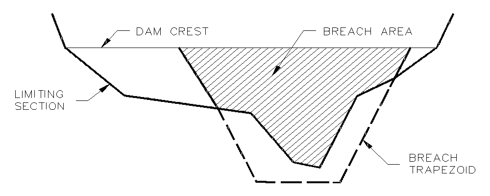
Figure: The breach (shaded area) is the area of the trapezoid inside the limiting cross section.

Flow calculations

Once the breach geometry has been computed the flow can be calculated.

The flow over the dam crest and the flow through the breach are often quite different with respect to water depth, velocity, and flow state. At the breach the water level is lower and the velocity is higher than at the dam crest. When the flow is drowned at the breach the flow at the crest may be either free overflow or drowned.

The flows through each structure are calculated separately using the upstream water level (h₁), the downstream water level (h₂) and the total flow (Q) from the last iteration. The flow over the crest structure and through the breach structure is calculated as described in section A.2.4 Structures (p. 295).

NWS DAMBRK dam breach methods

There are two NWS DAMBRK methods:

• Breach failure
• Piping failure

The first of these uses a weir type equation to determine the flow through the breach and the latter is based on an orifice type equation. Both methods rely on the user specifying the full development of the breach geometry as a function of time.

Breach failure

The flow through the trapezoidal breach is given by

\[ Q = c_v k_s\left[c_{weir} b \sqrt{g(h-h_b)}(h-h_b) + c_{slope} S \sqrt{g(h-h_b)}(h-h_b)^2\right] \]

Equation: Discharge through trapezoidal dam breach combining weir and slope flow components.

where

bthe width of the breach bottom g          is acceleration due to gravity h          upstream water level (reservoir water level) h_b          level of breach bottom S          side slope of breach c_weir is weir coefficient for horizontal part (=0.546430) c_slope is weir coefficient for slope part (=0.431856) c_v is correction coefficient for approach sections. This coefficient compensates for the loss in energy due to the inflow contraction. k_s is correction coefficient due to submergence.

The weir coefficients have been made non-dimensional e.g.

\(c_{weir}\sqrt{g} = 0.546430\sqrt{9.81(m/s^2)} = 1.7115(m^{1/2}/s) = 3.1(ft^{1/2}/s)\)

The correction coefficient for the approach section is determined through

\[ e = \frac{\text{min}\left(Q_{\text{left}}, Q_{\text{right}}\right)}{\text{max}\left(Q_{\text{left}}, Q_{\text{right}}\right)} \]

Equation: Brater coefficient for approach section flow balance in dam breach calculations.

where

c_B is non-dimensional coefficient (= 0.740256) termed the Brater coefficient W_R is reservoir width given by the undestroyed crest length. h_b,term is the terminal level of the breach bottom. The minimum level in the time series file. Q~p ~is discharge through the breach in the previous iteration.

The submergence correction is determined through

\[ k_s = \max\left(1 - 27.8\left(\frac{h_{ds}-h_b}{h-h_b} - 0.67\right)^3, 0\right) \]

Equation: Submergence correction factor for dam breach accounting for downstream drowning effect.

where h_ds is the downstream water level.

Piping failure

The flow through a piping failure is given by

\[ Q = c_{orifice}A\sqrt{2g\left(h -\text{max}\left(h_{p}, h_{ds}\right)\right)} \]

Equation: Discharge through an orifice as function of orifice area and available head difference.

where

c_orifice   Orifice coefficient (= 0.599769)

AFlow area in pipe given by

\[ A = b(h_{pt} - h_b) + S(h_{pt} - h_b)^2 \]

Equation: Cross-sectional area in a pressurized pipe from pipe geometry and water depth.

h_pt   Top of pipe

h_b   Bottom of pipe

h_p   Centre line of pipe given by

\[ h_{p}=\frac{(h_{p t}+h_{b})}{2} \]

Equation: Depth at pipe centerline for dam breach modeling.

The pipe may collapse either due to the top of the pipe reaching the crest level or if the water level upstream is not high enough to maintain pipe flow. The criteria for the latter is given by

\[ h<\frac{3}{2}(h_{p t}-h_{b})+h_{b} \]

Equation: Water level criterion for pipe failure in dam breach model.

Once the pipe has collapsed the flow is calculated based on the breach flow equations.

Crest flow

The flow over the crest of the dam is given by

\[ Q~=~k_{s}c_{w e i r}b_{c}\sqrt{g(h-h_{c})}(h-h_{c}) \]

Equation: Discharge over dam crest from weir flow formula.

where

h_c   the crest level

b_c   the remaining crest length (perpendicular to the flow)

and the submergence correction given by

\[ k_{s}~=~\mathrm{max}\Bigl(1\!-\!27.8\Bigl(\!\frac{(h_{d s}\!-\!h_{c})}{(h\!-\!h_{c})}\!-\!0.67\Bigr)^{3},0\Bigr) \]

Equation: Submergence correction factor for weir overflow flow in dam breach.

Temporal development of breach geometry

Once the failure has initiated the temporal development of the breach will be read from a time series. This time series must contain values for

• The breach bottom.
• The breach side slope.
• The breach bottom width.

Further if piping failure is used the time series must also contain

• The upper level of the pipe.

This is illustrated in the definition of term used in the NWS DAMBRK routines.

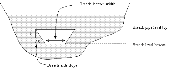
Figure: Definition of term used in the NWS DAMBRK routines.