Flood Plains
When the water level in a river is high, the river will in some places increase dramatically in width as the water flows into relatively large flat areas next to the natural river bed. These areas are called flood plains, and they require care when modelling the river flow since the water typically flows much slower in flood plains than in the natural river bed.
Description of flow over flood plains can be achieved with several different types of model schematisations depending on the topography of the flood plain and the nature of the flow.
In spilling areas natural levees are formed along the river by sedimentation due to the abrupt reduction in flow velocity of the entering water. In predominantly drainage areas, these levees are not present. The principal difference between the two situations is shown in the cross section view of the drainage area (left) and spilling area (right)
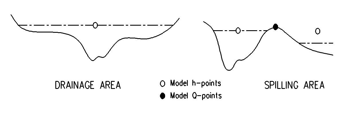
Figure: Cross section view of the drainage area (left) and spilling area (right).
This schematisation of the flood plain may not be adequate if sediment transport is to be calculated; especially where the hydraulic resistance in the flood plain is significantly different from that in the channel. This is because the sediment transport is very sensitive to the value of the velocity, and the average velocity across a cross section will not be representative of the actual velocity in the flood plain. For this situation, the river and flood plain may be schematised separately using two or more parallel model branches connected by broad crested weirs.
In a typical drainage area, it is generally reasonable to assume that the water level is the same in the river and on the flood plain. The flood plain storage can thus be included directly in the modelled river cross section through the cross section width, and only one model h-grid point is required to determine the water level over the whole area.
In a typical spilling area, the water levels in river and flood plain might differ due to separation by a levee. One h-grid point at each side of the levee is thus required to describe the situation. Between the two h-grid points a Q-grid point is placed that represents the discharge over the levee. A weir equation is applied to describe the magnitude of the discharge. This discretisation is shown in the right hand part of the cross section view of the drainage area (left) and spilling area (right). A schematic plan view of such a discretisation is shown in the top view of one possible method of discretisation with flood cells.
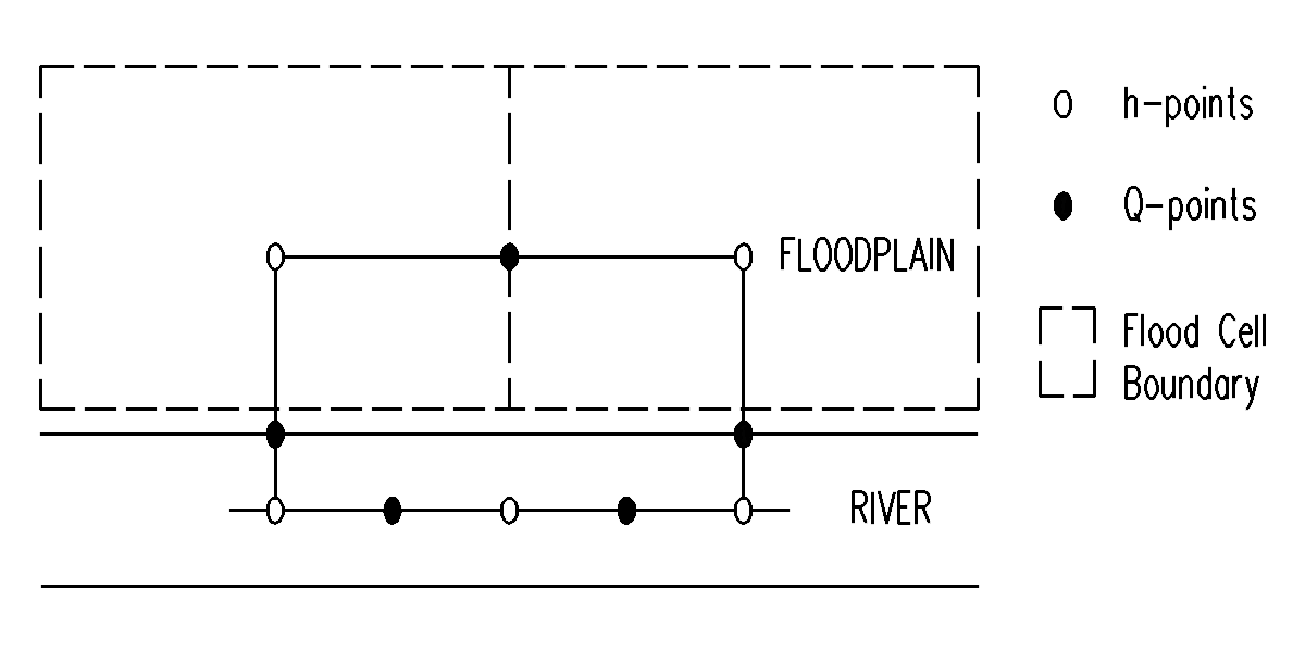
Figure: Top view of one possible method of discretisation with flood cells.
If water flows along the flood plain then the momentum equation must also be modified. The flood plain is divided into cells with one h-grid point describing the water level in each cell. Over the flood plains, flow can take place from one cell to the next. This is described by introducing a model branch between the cells (see the top view of one possible method of discretisation with flood cells). The boundaries between the cells are normally chosen along natural elevations such as roads or railway embankments. Where such features do not exist or are not sufficiently significant to merit explicit representation (but may be implicit in the flood plain roughness), the Saint-Venant equations can be applied. The water surface slope will then vary linearly between h-points.
If no cross section data exists on the flood plain, the cross section parameters can be derived from a storage-elevation relationship. From the storage-elevation relationship, the storage volume of the cell (denoted by V) can be determined as a function of elevation, and the area of the cross section in the flood cell can be approximated as:
Equation: Cross-sectional area derived from storage-elevation relationship in flood plain cells.
where, L is shown in the side view of a Section showing cell discretisation around a road.
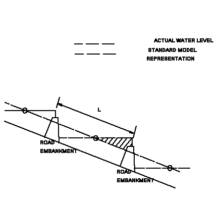
Figure: Side view of a Section showing cell discretisation around a road.
This will represent a measure for the average cross section along the flood plain. The average resistance radius can similarly be approximated with:
Equation: Average resistance radius for a flood plain storage cell.
When spilling starts, huge flows of water may suddenly be generated across a wide weir, possibly causing numerical instabilities. This problem can be overcome by giving the levee along the river a V-formed shape in the mathematical description, see the side view of a V-formed levee.
This ensures that spilling starts gradually instead of instantaneously over the whole section. This corresponds, in fact, to the situation often encountered in nature, where irregularities in levee height cause the spilling to start as trickles at certain positions along the levee.
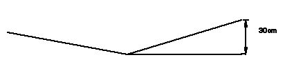
Figure: Side view of a V-formed levee. The V-form ensures that water gradually flows over the levee.
The computed water level in the cell is not representative for all locations within the cell, but is an average as shown in the side view of a Section showing cell discretisation around a road. To interpret the model results, the computed water level should be transformed into an average depth of inundation within the cell as given by:
Equation: Average inundation depth in flood plain cell from volume and surface area.