Numerical Schemes
The schemes used to solve the Saint-Venant equations are based on an implicit finite difference scheme developed by Abbott and Ionescu (1967). Here, we provide an overview of the schemes. Details are given in Appendix A.2.
A computational grid of alternating q-grid points (discharge) and h-grid points (water level) points is used as illustrated in the reach section with h- and q-grid points, on which the Saint-Venant equations are solved (see also Section A.2.1). The computational grid is automatically generated on the basis of the user requirements. q-grid points are placed midway between neighbouring h-grid points and at structures, while h-grid points are located at cross sections, or at equidistant intervals in between if the distance between cross sections is greater than a user-specified maximum distance. The sign of the discharge is defined by convention as positive in the positive x-direction (increasing chainage).
In MIKE+ setups, the maximum distance between grid points is calculated automatically from the height of the reach, its slope, etc. for reaches without a user-defined topography. Lower reaches will have smaller distances between grid points to ensure stability.
The conservation of mass equation, Equation (4.1a), is approximated on h-grid points and the conservation of momentum, Equation (4.1b), is approximated on q-grid points.
Equations (4.1a) and (4.1b) are converted into a system of coupled equations, which are solved to find the water depth and discharge throughout the network. The solution algorithm is referred to as the double sweep algorithm. See 1 for details.
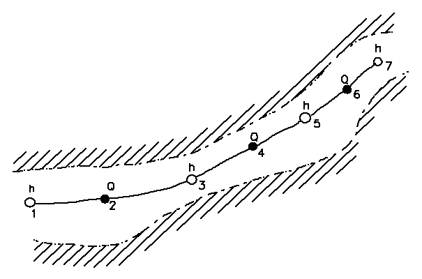
Figure: Reach section with h- and q-grid points, on which the Saint-Venant equations are solved.
There are different methods for approximating the momentum equation. The MIKE 11 and MIKE+ interfaces give the user control over which approximation method to use. See Appendix A.2.1.2 for details on how the different methods are implemented.
In MIKE 11, the Diffusive wave approximation and the Kinematic wave approximation can be selected as methods for solving the momentum equation.
The diffusive wave description ignores the inertia terms and is therefore suitable for 1) backwater analyses, 2) cases where the bed resistance forces dominate, and 3) for slowly propagating flood waves where the change in inertia is negligible. It is not normally suitable for tidal flows.
This formulation still ensures a backwater description through the ∂h/∂x term. For stability reasons the ∂h/∂x term is dampened in the solution, which means that only relatively steady backwater phenomena (compared to the time step) are resolved.
In the kinematic wave approximation, a balance between the friction and gravity is assumed and the discharge becomes a function of upstream water level alone. This means that the kinematic wave approach cannot simulate backwater effects. Thus this description is appropriate for relatively steep rivers without backwater effects.
The diffusive and kinematic wave approximations are simplifications of the full dynamic descriptions. They are implemented to offer improved computational efficiency, but should only be used when the omitted terms have insignificant influence. When there is any doubt it is better to use the full dynamic description or trials should be undertaken to establish the difference between alternative methods, and advice sought from experienced persons. It is very important to have a solid understanding of the influence of the different terms.
None of the three wave descriptions includes detailed hydraulic descriptions of hydraulic jumps. However, the chosen formulations ensure a correct description upstream and downstream of the jump.
Multiple threads can influence results
The underlying numerical scheme uses a matrix equation solver that supports multiple CPUs (meaning that the solver will take advantage of all available cores in a computer).
Please note that if more than one thread is used, then the matrix solver does not guarantee the same result every time the solver is run (the reason is that the order of steps in the algorithm can be different). The difference in the results is normally so small that is can safely be disregarded. However, if the setup is unstable and conditions are unfavourable, then very small differences can be amplified and the results can differ markedly from simulation to simulation. Thus, if a situation is encountered where results differ from simulation to simulation, then it is recommended running the simulation with only one thread.
Please also note: If a situation is encountered where results differ markedly from simulation to simulation, then the result can most likely not be trusted, even if they are reproducible with only one thread. The real solution to the problem of different results from simulation to simulation is thus to ensure that the simulation is stable.
-
Abbott, M.B. and Basco, D.R.: Computational Fluid Dynamics, an introduction for engineers. Longman Scientific & Technical, 1989. ↩