Processing of Raw Data¶

Cross sections specified by raw data are automatically converted into processed data (this is called processing). Processing creates processed data tables, which are used by the engine for flow computations. The processed data tables contain the following columns

h = water level or depth, [m] b_s= storage width, [m] A_fl = flow area, [m²] F = resistance number, R = hydraulic radius, [m]

The processing specification contains the minimum and maximum water levels within which to process data, and optionally the number of processed levels to create. The processed levels can either be generated automatically, in which case the level spacing will be decided by the processing algorithm, it can be an equidistant number of levels, or the processed levels can be provided as part of the processing specification.

For each processing level the processed data table column values are calculated. The storage width b_s and the flow area A_fl are computed directly from the geometry of the cross section. The resistance number F and hydraulic radius R depend on the resistance specification of the cross section and are described in detail in the following sections.

Urban (MIKE+)River (MIKE 11 / MIKE HYDRO)

In MIKE+ (Collection System) by default processes it cross sections using 50 equidistant levels.

For MIKE 11 processing can be performed by the cross section editor and stored in the xns11 file. If processed data is not stored in the xns11 file, the engine processes cross sections using the same algorithms as the cross section editor.

Relative resistance and effective area¶

When relative resistance is specified for a cross section, the effect of the relative resistance number, r, is included in the hydraulic radius R and the flow area A_fl, while the processed resistance numbers F by default are constant 1 for all levels.

If the hydraulic radius type used is either “Resistance Radius” or “Hydraulic Radius, Effective Area”, an effective area is calculated. The effective area tries to take into account the amount of water that due to resistance is not giving any contribution to the momentum, and is used in the Momentum Equation (4.1b), instead of the geometric area.

The effective flow area, A_e, for a given water level is defined as:

\[ A_e = \int_0^B \frac{y}{r} db \]

Equation: Effective flow area accounting for spatial variation in resistance number.

where, y is the local water depth and B is the width of the cross section at the given water level.

Looping over all line segment in the cross section profile (which equals the number of raw (x,z) values minus one), this converts to a sum on the form

\[ A_{e}=\sum_{i}\!\left(\frac{A_{i}}{r_{i}}\right) \]

Equation: Effective flow area weighted by inverse of relative resistance across cross section segments.

where A_i is the area above the i’th line segment up to the current water level, and r_i is the relative resistance specified for the line segment.

In case the relative resistance value is constant 1 along the entire cross section profile, the effective area will equal the geometric area.

The effect on the hydraulic radius will be described in the next section.

Hydraulic radius¶

The hydraulic radius is a measure of the effect of the wall/bed resistance on the water volume. The larger the hydraulic radius, the larger amount of water is affected by each metre of the wall; there is thus less friction and the reach will convey water more efficiently.

The hydraulic radius is traditionally defined as

\[ R_{h}=\frac{A}{P} \]

Equation: Hydraulic radius computed as the ratio of cross-sectional area to wetted perimeter.

where A is the cross section and P is the length of the wetted perimeter. The wetted perimeter is the portion of the cross section perimeter that is currently wet.

The traditional definition of the hydraulic radius has some properties that are not desirable in all situations. Therefore a number of variations exist, and the hydraulic radius used can be one of three different types:

Resistance radius
Hydraulic radius, effective area
Hydraulic radius, total area

The two types of hydraulic radii, effective area and total area, are alike except when specifying a relative resistance number which varies along the cross section profile, either as distributed resistance numbers or using flow bank zones.

The hydraulic radius is calculated from the raw data. The following sections describe how the hydraulic radius is calculated.

Resistance radius¶

The resistance radius at a given water level is calculated as (¹):

\[ \sqrt{R_*} = \frac{1}{A}\int_0^B y^{3/2} db \]

Equation: Resistance radius calculated as flow-area-weighted average of local water depth.

where, y is the local water depth, A is the flow area and B is the width of the cross section at the given water level.

This formulation ensures that the resistance number is almost independent of the water depth in cases with significant effects from the flow bank zones.

Relative resistance¶

If relative resistance is specified, the flow area in Equation the resistance radius calculated as flow-area-weighted average of local water depth is replaced by the effective area, and it is updated to read:

\[ \sqrt{R_*} = \frac{1}{A_e}\int_0^B \frac{y^{3/2}}{r} db \]

Equation: Effective resistance radius weighted by depth to the 3/2 power across the cross-section.

In case the relative resistance number is constant over the cross section, Equation the effective resistance radius weighted by depth to the 3/2 power across the simplifies to Equation the resistance radius calculated as flow-area-weighted average of local water depth.

Hydraulic radius for relative resistance numbers¶

When relative resistance is specified, the hydraulic radius is calculated based on a parallel channel analysis where the total conveyance, K, of the cross section at a given elevation is equal to the sum of the conveyances of the parallel channels. The parallel channels of a cross section are defined as those parts of the cross section where the resistance number remains constant. We have

\[ K = \sum_{i = 1}^{N}K_{i} \]

Equation: Total conveyance calculated as the sum of conveyances in parallel sub-channels.

where N is the number of parallel channels.

The parallel channel analysis is based on a Manning’s n formulation, hence:

\[ \frac{AR^{2/3}}{n} = \sum_{i=1}^N \frac{A_i R_i^{2/3}}{n r_i} \]

Equation: Combined Manning conveyance for parallel channel analysis.

Setting A equal to either the effective flow area as given by Equation the effective flow area weighted by inverse of relative resistance across cross or the total flow area, we get the general formula:

\[ R_h = \left(\frac{1}{A}\sum_{i=1}^{N}\left(\frac{A_i^{5/3}}{r_i P_i^{2/3}}\right)\right)^{3/2} \]

Equation: Harmonic mean hydraulic radius computed from parallel channel flow properties.

where, P_i is the wetted perimeter of the parallel channel. P_i does not include the interface between adjoining parallel channels, i.e. a zero shear interface has been adopted.

Resistance Radius vs. Hydraulic Radius¶

The choice between R_* or R_h should be based on

which factor appears to be the most appropriate from a hydraulic aspect, and
which factor is normally used in local practice so that conventional bed resistance numbers can be used with confidence.

For a technical analysis Lundgren and Jonsson, ² present a comparison of five different methods for determining the shear stress distribution over the bed of a shallow channel.

To highlight the differences between R_* and R_h the following example is used. Consider the cross section shown in the cross Section used in the comparison of resistance radius $R*$and hydraulic radius $R_{h}$. In the case of a constant relative resistance of 1.0 over the cross section, the conveyance calculation for resistance radiusand hydraulic radiusfor both total gives the values of R_* and R_h (Case 1), and their corresponding conveyance, K, (defined here as AR^2/3) at selected water levels.

Table: Conveyance calculation for resistance radiusand hydraulic radiusfor both total and effective area.

Elev [m]	Area [m 2 ]	R * [m]	K	Rh[m] Case 1	K	Rh[m] Case 2	K
100.0	0.0	0.00	0	0.00	0	0.00	0
103.0	101.7	2.19	171	1.89	155	1.89	155
106.0	306.3	4.41	824	3.27	675	3.27	675
106.1	344.6	3.85	846	0.89	319	2.98	714
107.0	697.1	2.95	1434	1.74	1009	2.62	1325
108.0	1104.8	3.46	2527	2.64	2110	3.18	2389
110.0	1970.5	5.03	5780	4.36	5259	4.66	5498
113.0	3395.0	7.58	13100	6.75	12126	6.93	12340

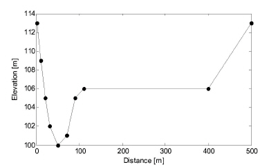
$Cross Section used in the comparison of resistance radius $R*$and hydraulic radius $R_{h}$$

Figure: Cross Section used in the comparison of resistance radius $R*$and hydraulic radius $R_{h}$.

The comparison of the conveyance values, shown in the plot of conveyance with surface elevation, provide a guide as to how the hydraulic capacity of the section varies with the water level. The figure shows that:

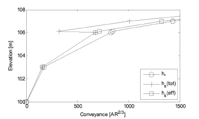
Plot of conveyance with surface elevation

Figure: Plot of conveyance with surface elevation.

R_* allows a smooth transition in the conveyance of the channel as the over bank region becomes flooded, while R_h causes a sharp, incorrect decrease in the conveyance;
The conveyance in the deep sections is considerably greater for R = R_*. This is because R_* can over-estimate the conveyance for very deep and narrow cross sections as it does not fully take into account the friction from the cross section sides as does the R_h formulation.

The conveyance curve for the R_h case can be improved by separating the cross section illustrated in the cross Section used in the comparison of resistance radius $R*$and hydraulic radius $R_{h}$ into two parallel channels (main channel and over bank channel) separated by an apparent third channel of zero width at a distance of 110 m along the x axis. This can be done by specifying a change in relative resistance where the two parallel channels meet - which in reality is the norm as the over bank channel typically would have a higher resistance than the main channel. R_h - Case 2 in the conveyance calculation for resistance radiusand hydraulic radiusfor both total is in the case of a r_r of 1.1 specified for the channel of zero width, and r_r of 1.0 elsewhere. (This has the effect of splitting the section into three parallel channels with the conveyance of the middle channel being zero.) As can be seen in the plot of conveyance with surface elevation a much improved conveyance -elevation relationship results.

In general, R_* is suited to sections with significant variations in shape such as over bank flow paths, while R_h, with no variation of r_r (i.e. one parallel channel) is more appropriate for very deep and narrow uniform sections. For R_h, where over bank flow paths occur, adjustment of r_r should be made to invoke the parallel channel analysis facility as described above. For wide sections with little variation in depth, R_* and R_h will not differ greatly.

River (MIKE 11 / MIKE HYDRO)

In the cross section editors processed Data menu a conveyance column is shown where the conveyance is defined as follows:

For Manning's number

\[ K = r_f A R^{2/3} \]

Equation: Conveyance for Manning's formulation expressed as resistance factor times flow area and hydraulic radius term.

where r_f is the resistance factor.

Calculation of processed resistance numbers¶

For cross sections where the resistance number is varying over the cross section profile, the calculation of processed resistance numbers for a given water level is based on a similar parallel channel analysis as in previous sections. For a given water level, the following procedure takes place:

The resistance numbers are converted to relative resistance numbers.
- The resistance number with the largest resistance is found, and all resistance numbers are scaled with that, such that all resistance numbers are in the range from 0 to 1. Note that for resistance formulations where the largest resistance number gives the smallest resistance, like Manning’s n formulation, the number found is the smallest resistance number. For Manning’s M and n and Chezy formulation, the largest resistance number is found like:

\[ M_{m a x}~=~\mathrm{max}(M_{i}), \frac{1}{n_{m i n}}~=~\mathrm{max}\Big(\frac{1}{n_{i}}\Big), C_{m a x}=\mathrm{max}(C_{i}) \]

Equation: Maximum resistance numbers for Manning and Chezy resistance formulations.

and the relative resistance numbers are then

\[ r_{i}=\frac{M_{i}}{M_{m a x}},\quad r_{i}=\frac{n_{m i n}}{n_{i}},\quad r_{i}=\frac{C_{i}}{C_{m a x}} \]

Equation: Relative resistance numbers normalised by their maximum or minimum values.

The effective area and hydraulic radius are calculated as described in Section 3.4.1 and 3.4.2 using these relative resistance numbers. The hydraulic radius using the effective area, i.e. it is either “resistance radius”, or “hydraulic radius, effective area”. These will be denoted A_e and R_e.
The area and hydraulic radius are calculated once more, this time using a constant relative resistance of 1 on the entire cross section, giving a total area and radius. These will be denoted A_tot and R_tot.
The effective resistance number for the given water level is the maximum resistance scaled with the effective vs. total conveyance fraction:

\[ M_p = M_{max} \frac{A_e R_e^{2/3}}{A_{tot} R_{tot}^{2/3}} \]

Equation: Effective Manning resistance scaled by the ratio of effective to total conveyance for a given water level.

\[ n_p = n_{min} \frac{A_{tot} R_{tot}^{2/3}}{A_e R_e^{2/3}} \]

Equation: Effective Manning resistance number scaled by conveyance ratios for variable water depth.

\[ C_{p}~=~C_{m a x}\frac{A_{e}\sqrt{R_{e}}}{A_{t o t}\sqrt{R_{t o t}}} \]

Equation: Effective Chezy resistance coefficient scaled by effective versus total conveyance.

Manual modification of the resistance factor¶

The variation of resistance number with elevation is stored in the resistance number column of the processed data. These can be modified by hand, if another vertical variation of the resistance number is desired.

If the cross section specifies relative resistance, the resistance number is a resistance factor. It is by default defined as 1.0 for all water levels. When a resistance number is required by the engine, the global constant resistance number is multiplied by this resistance factor. The effect of this resistance factor on the resistance number is dependent on the friction formulation used. In case of Chezy and Manning’s M, an increase in the resistance factor will cause a decrease in resistance, while for Manning’s n an increase in the resistance factor will increase the resistance.

Processing of user specified cross sections from MIKE+¶

Urban (MIKE+)

MIKE+ (Collection System) user-specified cross sections are processed with 50 equidistant levels, covering the bottom to the top of the cross section. For open cross sections, the top is defined by the lowest of the two bed levels.

For open cross sections, a top slot is not set by default, meaning that if the water level exceeds the level of one of the bed sides, the simulation will stop. It is possible to modify the default behaviour and extrapolate the processed cross section data upward by from the DHIAPP.INI file.

For closed cross sections, a top slot is set: an additional 50 levels are added to the existing processed levels. The top few levels of the existing 50 levels are updated to assure a smooth transition from the first 50 levels to the 50 levels of the top slot levels. On top of the 100 levels, a top slot is added that extends to infinity but which returns constant values for cross section area, width and hydraulic radius. The constant values are taken from the processed data at the level where the top slot begins (Constant ARW top slot, see Section A.4.6).

Conveyance modifications¶

To ensure computational stability, the cross section conveyance should monotonically increase or be constant for increasing water levels.

This is normally not the case with pipes; for pipes, the values of conveyance drop in the region near the top of the cross section.

For such cases, when raw data is used, the hydraulic radius is adjusted as part of the processing so that the limiting conveyance for the cross section corresponds to the actual conveyance value for the full profile. the corrected conveyance curve and the corrected hydraulic radius shows the effect of the correction on the conveyance and hydraulic radius for a circular pipe cross section with a radius of 1.5 m.

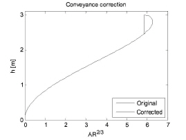
Corrected conveyance curve

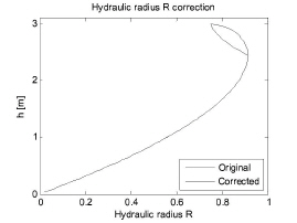
Figure: Corrected conveyance curve.

Corrected hydraulic radius

Figure: Corrected hydraulic radius.

When closed cross section processed data are used or manually edited, attention should be paid to the upper region of the profile, so that decreasing conveyance is avoided.

When using the cross section editor this is accomplished by monitoring the conveyance column in the processed data table; the conveyance should be monotonically increasing with increasing water level.

Engelund, F.: Hydraulic resistance of alluvial streams. ASCE, Vol. 92, No. Hy. 2, 1966. ↩
Lundgren, H. and Jonsson, I.G.: Shear and velocity distribution in shallow channels. ASCE, Vol. 90, No. HY1, pp. 1-21, 1962. ↩