Time Area Surface Runoff Model
Concept
In the Time-Area surface rainfall-runoff method the amount of runoff is controlled by the initial loss, the size of the contributing area and by a continuous hydrological loss. Moreover a snow storage may also be added to the computation.
The shape of the runoff hydrograph is controlled by the concentration time and by the time-area (T-A) curve. These two parameters represent a conceptual description of the catchment reaction speed and the catchment shape.
Input data
Model specific data
Impervious area [%] represents the fraction of the catchment area considered to contribute to the runoff.
Hydrological parameters
Initial Loss [m] defines the precipitation depth required to start the surface runoff. This is a one-off loss, comprising the wetting and filling of catchment depressions.
The default value is 6.00 10-4 m.
Hydrological Reduction [-] is a runoff reduction factor accounting for water losses caused by e.g. evapo-transpiration, imperfect imperviousness, etc. on the contributing area.
The default value is 0.90.
Time/Area Curve accounts for the shape of the catchment layout, determines the choice of the available T/A curve to be used in the computations.
Three predefined types of the T/A curves are available:
-
rectangular catchment
-
divergent catchment
-
convergent catchment
Table: Predefined types of T/A curves.
| Curve type 1 Time [-] | Curve type 1 Area [-] | Curve type 2 Time [-] | Curve type 2 Area [-] | Curve type 3 Time [-] | Curve type 3 Area [-] |
|---|---|---|---|---|---|
| 0 | 0 | 0 | 0 | 0 | 0 |
| 1 | 1 | 0.1 | 0.12 | 0.1 | 0.01 |
| 0.2 | 0.28 | 0.2 | 0.04 | ||
| 0.3 | 0.47 | 0.3 | 0.08 | ||
| 0.4 | 0.61 | 0.4 | 0.15 | ||
| 0.5 | 0.72 | 0.5 | 0.24 | ||
| 0.6 | 0.8 | 0.6 | 0.35 | ||
| 0.7 | 0.87 | 0.7 | 0.47 | ||
| 0.8 | 0.93 | 0.8 | 0.62 | ||
| 0.9 | 0.98 | 0.9 | 0.8 | ||
| 1 | 1 | 1 | 1 |
The user-defined T/A curve can be specified, thus allowing correct description of irregular catchments.
The default T/A type is a pre-computed curve type 1.
From the MIKE 11 interface it is not possible to enter a user-defined T/A curve. The choice can only be made between one of the three predefined T/A curves.
Time/Area Coefficient [-] is used in a formula introduced in order to cover curve shapes “in between” the three standard ones (and outside). The formula has been suggested by Nittaya Wangwongwiroj at AIT. The curves “in between” are specified by giving the Time Area Coefficient.
(7.32) 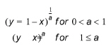
Figure: Time-area coefficient formula for catchment shapes between the standard types.
Table: Variables in the time-area coefficient formula.
| y | Accumulated dimensionless area |
| x | Dimensionless concentration time |
| a | Time area curve coefficient |
The predefined curves 1, 2, and 3 as described above respectively correspond to a coefficient of 1, 0.5 and 2. Below is seen a plot of the curves.
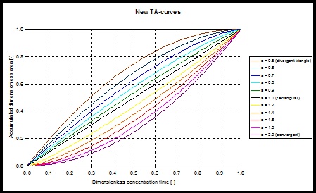
Figure: Example of T/A curves.
The Time Area coefficient method is not available for the MIKE 11 interface.
Concentration Time [s] defines the time required for the flow of water from the most distant part of the catchment to the point of outflow.
The default value is 420 seconds.
Loss Recovery Rate [m/s] defines the rate to recover the initial loss during dry periods. Instead of this constant rate, an evaporation time series can be provided.
The default value is 5 10-5 m/h.
Snow melt coefficient [m/°C/s] defines the rate of snow melting when temperature exceeds zero degrees Celsius.
Runoff computation
Snow storage computation
Snow can accumulate when the temperature is inferior or equal to zero degrees Celsius (\(T\leq0^{\circ}C\)). During warmer periods, when temperature exceeds zero degrees Celsius (\(T>0^{\circ}C\)), the snow storage melts at a rate given by the snow melt coefficient. The snow storage computation will be performed only if a temperature time series is provided for the catchment.
During storing periods, or \(T\leq0^{\circ}C\) the snow will accumulate without limit. If the temperature is below zero degrees Celsius, it is assumed that the entire rainfall will be stored as snow.
During melting periods, or \(T>0^{\circ}C\) the snow will melt and therefore contributes to the surface runoff at rate given by the snow melt coefficient.
The snow module is the first process occurring after rainfall, therefore all others losses will be computed afterwards.
Effective precipitation computation
The simulated hydrologic processes account for specific losses. The runoff starts after the rain depth has exceeded the specified initial loss for the catchment. The remaining precipitation is called effective precipitation, defined generally as:
Equation: Effective precipitation accounting for initial losses.
Where:
Table: Variables in the effective precipitation equation.
| \(I_{eff}(t)\) | Effective precipitation at time t |
| \(I(t)\) | Actual precipitation at time t |
| \(I_{w}(t)\) | Wetting loss at time t |
The actual precipitation, \(I(t)\), is assumed to be uniformly distributed over the individual catchments. Otherwise, it may vary as a random time function.
The wetting, \(I_{w}(t)\), is a discontinuous loss, also called initial loss. When the precipitation starts, a part of the precipitation is used for wetting of the surface if the surface is initially dry. When the surface is wet, the wetting loss, \(I_w\), is set to zero. This is summarised in the following expression:
Equation: Wetting loss (initial abstraction) during precipitation limited by surface saturation and intensity.
Where:
Table: Variables in the surface runoff routing equation.
| \(I(t)\) | Actual precipitation at time t |
| \(I_{w}(t)\) | Wetting loss at time t |
| \(y_{w}\) | Wetting depth |
| \(I(t)\) | Accumulated depth at time t |
Surface runoff routing computation
The continuous runoff process is discretised in time by the computational time step \(\Delta t\). The assumption of the constant runoff velocity implies the spatial discretisation of the catchment surface to a number of cells in a form of concentric circles with a centre point at the point of outflow. The number of cells being equals to:
Equation: Number of time-area cells computed from catchment concentration time and computational time step.
Where:
Table: Variables in the number of time steps equation.
| \(t_{c}\) | concentration time [s] |
| \(\Delta t\) | simulation time step [s] |
The 1D engine calculates the area of each cell on the basis of the specified time-area curve or coefficient. The total area of all cells is equal to the specified impervious area.
A time-area curve characterises the shape of the catchment, relating the flow time i.e. concentric distance from the outflow point and the corresponding catchment sub-area. Irregularly shaped catchments can be more precisely described by the user-specified T/A curves or coefficient.
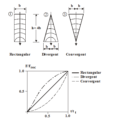
Figure: The three predefined time/area curves available.
The runoff stops when the accumulated rain depth on the whole catchment surface regresses below the specified initial loss for the catchment.
At every time step after the start of the runoff, the accumulated volume from a certain cell is moved to the downstream direction. Thus, the actual volume in the cell is calculated as a continuity balance between the inflow from the upstream cell, the current rainfall (multiplied with the cell area) and the outflow to the downstream cell. The outflow from the most downstream cell is actually the resulting surface runoff hydrograph.
To account for the specified hydrological reduction, the runoff from the impervious surface is reduced by the catchments hydrological reduction factor.
Multiple-event simulations
If the Time Area Surface Runoff Model is used for a continuous simulation of multiple rainfall, a special solution can be applied for the simulation of dry periods between the consecutive events. The solution accounts for the loss of water caused by drying out of the initial loss (representing wetting and surface storage), i.e. allowing the occurrence of the initial loss at the beginning of each simulated event, in accordance with reality.
In this context, start of a dry period is defined if two conditions are fulfilled simultaneously:
- No rainfall: all connected rain gauges show no rain.
- No runoff: the runoff has fallen to zero from all catchments included in the simulation.
At the start of a dry period, the initial loss storage would be fully or partially filled up, the latter being the only case for small events of the total depth smaller than the initial loss storage depth. Recovery of the initial loss capacity, i.e. the process of surface drying is simulated as a constant “decay” rate, which replaces the actual evaporation. As a consequence of the recovery process, the initial loss storage would be fully or partially emptied, which depends on the actually applied loss recovery rate and the duration of the dry period.
The evaporation rate can be given as Initial Loss Rate or as an evaporation time series. If the actual evaporation is not explicitly specified in the simulation (i.e. Evaporation process activated – see INI file parameters – and evaporation time series specified), only a decay rate will be applied during dry periods.
The recovery process is only activated during dry periods, i.e. the evaporative action during rain events is neglected.